homework 11: the adventure of the 2001 dimensions

Watson, a distinguished-looking MD/PhD student who's recently returned from some field work in Afghanistan, comes to you with a problem. He says he was impressed by the lab meeting you gave on Wiggins' K-means analysis a couple of weeks ago. He's been working with a single cell RNA-seq data set from the glands of a langur monkey. Under the microscope, he sees, clear as day, 8 morphologically distinct cell types. But in his RNA-seq data, try as he may, he can't seem to find any intelligible differences in their gene expression patterns. He's convinced that the differences must lie in some of the 2001 neuron-specific sand mouse genes, but he's been unable to identify a meaningful clustering by K-means or other methods. He implores you to take a look at his counts data, which are based on 200 single cell RNA-seq experiments and in tidy format, with each gene as a column and each observation as a row. In the figure below, he shows you a heat map in which he's drawn horizontal white lines to separate his k=8 K-means clusters.

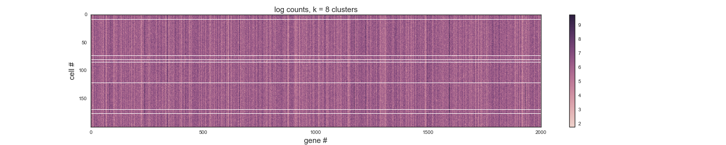You can 'open image in new tab' to make this figure bigger.

You have a hard time making heads or tails of Watson's K-means heat map. It looks like a mess, and it doesn't seem like the best way to plot clusters based on high-dimensional data. You're most familiar with 2D scatter plots like what Wiggins used in describing K-means results in his notebook, where it was easy to visualize how cells were clustered. If you can visualize the data similarly, you'll have an easier time homing in on Watson's problem. But you'll have to figure out a way to project Watsons's 2001-dimension data set down into two dimensions.

1. reproduce Watsons's K-means result

Modify the K-means clustering procedure you wrote for Wiggins' data so that it works in 2001 dimensions, not just 2. Run a reasonable number of iterations (20-100, or even better, test for convergence), starting from several different initializations; report the lowest total squared distance (best clustering) you find for K=8. It should be close to what Watson found using k = 8 clusters, where his clustering achieved a sum of the squared distance = 87378.2. He used the "fixed" K-means method from part 3 of hw09, with his data represented as log counts.

2. reduce the dimensionality

Write a Python function that uses singular value decomposition to find the principal components of the data set.

Plot all 200 cells in 2D PCA space using their projections onto the first two principal axes.

Was Watson right to expect 8 clusters? Plot the eigenvalues for each component, and justify why you're pretty sure it would be hard to find any other clusters in the data set. The eigenvalues from a simulated negative control data set, where there were no cell types and no correlations between any of the genes, should factor into your answer.

Based on the eigenvector loadings, how many genes appear to influence cell type identity? Explain.

3. check the clustering

Plot the data in 2D principal component space, and color each point according to the cluster identities from part 1. You should find that K-means is missing the mark.

Offer an explanation of what might be going wrong, and find a way to cluster so that each cell appears properly assigned in PC space.

4. reconstruct the expression patterns

Reconstruct the original data set using only the projected data and eigenvectors for the first 2 principal components. Visualize the data using a heat map. Do the clusters now look more obvious? Why or why not?

allowed modules

My imports:

import numpy as np
import pandas as pd
import matplotlib.pyplot as plt

%matplotlib inline

So far in the course we've also now allowed scipy.stats, scipy.special, scipy.optimize, seaborn, and re, but you probably won't need them this week.

turning in your work

Submit your Jupyter notebook page (a .ipynb file) to the course Canvas page under the Assignments tab. Name your file <LastName><FirstName>_<psetnumber>.ipynb; for example, mine would be EddySean_11.ipynb.

We grade your psets as if they're lab reports. The quality of your text explanations of what you're doing (and why) are just as important as getting your code to work. We want to see you discuss both your analysis code and your biological interpretations.

Don't change the names of any of the input files you download, because the TFs (who are grading your notebook files) have those files in their working directory. Your notebook won't run if you change the input file names.

Remember to include a watermark command at the end of your notebook, so we know what versions of modules you used. For example,

%load_ext watermark
%watermark -v -m -p jupyter,numpy,matplotlib

notes

Remember that when using SVD, you want to center your data first by subtracting the mean of each column (variables) from the data. Without centering before SVD, the first principal component is merely proportional to the mean of the data over rows, and other components may be less interpretable as well. When using standard eigendecomposition, the covariance matrix, by virtue of its definition, will look the same on centered and non-centered data.

It's sometimes recommended to standardize, or whiten, your data by dividing each column by its standard deviation. This process ensures that variables with large intrinsic variance do not dominate components, which is essential when performing PCA with variables that do not share units. In other situations, however, the recommendation is less clear-cut, as differences in intrinsic variance between variables might be important features of the data. Indeed, in Watson's case, data whitening results in the loss of a few otherwise distinguishable clusters in PC space. Nevertherless, there is some risk in performing PCA on raw, non-standardized data, as significant covariations could be relegated to components with small eigenvalues (and thus ignored).

hints

The input data in w11-data.tbl are mapped read counts. You'll want to immediately transform them to log counts, as we've seen in K-means week. The RNA-seq count data are roughly lognormally distributed, whereas PCA is implicitly assuming Gaussian-distributed residuals, so PCA will behave better on log count data.

You might find that when using K-means in 2001 dimensional space, K-means sometimes creates an orphan cluster, a cluster that doesn't have any points assigned to it. If you encounter this, discard that K-means iteration and try a new initialization of random centroids.

np.linalg.svd() will conveniently return the decomposition with the $S$ matrix (and corresponding eigenvectors) sorted in descending order. In general, though, eigenvalues and eigenvectors might not come out sorted. To properly rank principal components as 1, 2, ..., p, you may need to make sure to sort the eigenvalues in descending order, together with their corresponding eigenvectors.

This pset was originally written by Tim Dunn for MCB112 in fall 2016.