week 08 Section

Notes by Jakob Heinz (2024)

Viterbi decoding

We'll start by walking through an example of a Viterbi decoding that I think is more intuitive than genomic data. This example is taken from the Viterbi algorithm wikipedia page.

Let's consider how Dr. Mittens might diagnose a patient. There are two states that the patient can have: Healthy and Fever. Unfortunately every thermometer in the greater Boston metro area has broken, so these states are hidden to Dr. Mittens. Dr. Mittens knows only what her patients tell her on a given day, namely: "I feel " + {"normal", "cold", "dizzy"}. From these observations, Dr. Mittens will try to reconstruct the patient's health state over the last few days. For example, if the patient was healthy, then had a fever for three days until they were healthy again, their hidden state would be "HHFFFHH". Dr. Mittens did very well on her MCAT and is an excellent physician, however she misses her college statistics classes terribly and has been reading too many Russian mystery novels, so she decides to employ a Hidden Markov Model approach to decode her patient's health state.

We have the following transition probabilities:

and the emission probabilities:

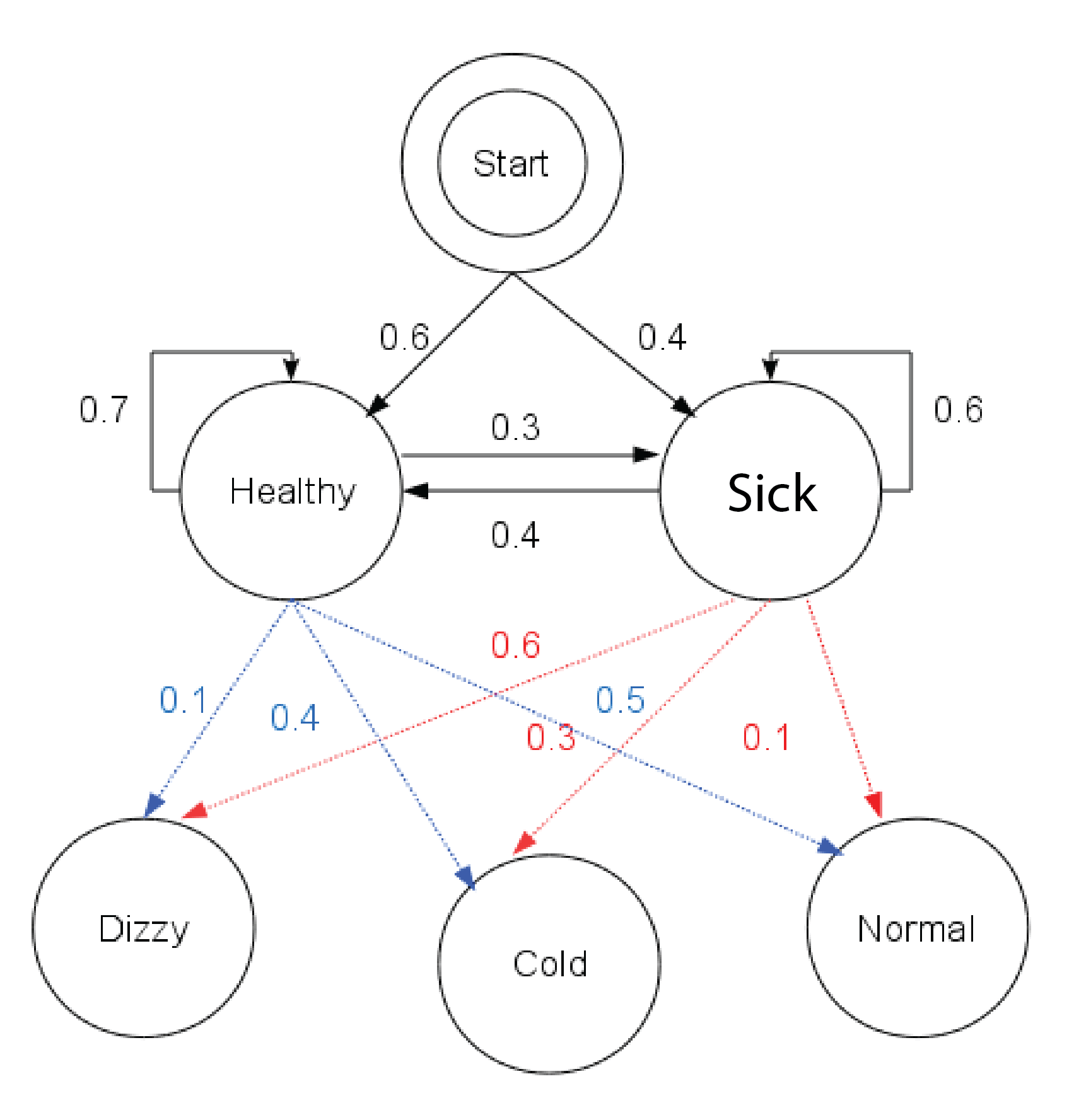
There's also the question of does the patient start in the healthy or fever state. Dr. Mittens assigns a 0.6 probability that the patient starts healthy and a 0.4 probability they start with a fever.

Here's diagram of this example (which comes from Reelsun on the Wikipedia page)

Dr. Mittens sees one of her patients three days in a row. The patient reports the following symptoms:

Day 1- Normal

Day 2 - Cold

Day 3 - Dizzy

Now it's up to Dr. Mittens to determine whether the patient was healthy or had a fever for each of these days. She begins by filling in her matrix so she can do her traceback.

she's opted to keep track of her traceback in a separate matrix, storing the index of where the maximum value came from

Important disclaimer! The following calculations should be done in log space. For the sake of interpretability, I kept them in probability space for our example. With so few calculations, underflow isn't an issue. If you're implementing this make sure to do so in log space!

Now let's fill in the first healthy and fever values. There's no emission probability for switching from healthy to fever yet, since we are coming from the start node, so these first two cells are simple:

and we update our traceback tracker with which state these values came from :

Now let's consider day2 where the patient felt cold:

first we'll fill out the healthy cell:

$$ max\begin{cases} P(x_1,x_2 = NC, \hat{\pi}(i-1)= H,\pi(i) = H) = 0.3 * 0.7 * 0.4 = \textbf{0.084}\ P(x_1,x_2 = NC, \hat{\pi}(i-1)= F,\pi(i) = H) = 0.04 * 0.4 * 0.4 = 0.0064\ \end{cases} $$

This tells us that the patient was most likely healthy on day2 if they were healthy on day1 given the observed symptoms of normal, then cold.

Now lets fill out the fever cell for day 2:

$$ max\begin{cases} P(x_1,x_2 = NC, \hat{\pi}(i-1)= H,\pi(i) = F) =0.3 * 0.3 * 0.3 = \textbf{0.027}\ P(x_1,x_2 = NC, \hat{\pi}(i-1)= F,\pi(i) = F) = 0.04 * 0.6 * 0.3 = 0.0072\ \end{cases} $$

So, if the patient was in the fever state on day2, it is more likely they were healthy day 1 and then had a fever day 2(HF), than a fever on both(FF)

lets update our matrix with what we've calculated:

We'll update our traceback matrix

Time to fill in our last cells for day3, where our patient reported feeling dizzy:

First the healthy cell:

$$ max\begin{cases} P(x_1,x_2, x_3= NCD, \hat{\pi}(i-1)= HH,\pi(i) = H) = 0.084 * 0.7 * 0.1 = \textbf{0.00588}\
P(x_1,x_2, x_3= NCD, \hat{\pi}(i-1)= HF,\pi(i) = H) = 0.027 * 0.4 * 0.1 = 0.00108\ \end{cases}$$

Then the fever cell:

$$ max\begin{cases} P(x_1,x_2, x_3= NCD, \hat{\pi}(i-1)= HH,\pi(i) = F) = 0.084 * 0.3 * 0.6= \textbf{0.01512}\
P(x_1,x_2, x_3= NCD, \hat{\pi}(i-1)= HF,\pi(i) = F) = 0.027 * 0.6 * 0.6 = 0.00972\ \end{cases}$$

Dr. Mittens has the filled out matrix now! We'll treat this as our end state as we've run out of observations. Let's take a look at the final matrix:

and the traceback matrix:

The highest value for our final day is 0.01512 at index (1,3), so this is where we start the traceback from. The path is denoted in bold font. Dr. Mittens has determined that the most probable decoding of her patient's hidden health state is healthy, healthy, fever. Now Dr. Mittens can go back to figuring out what happened to all the thermometers...

This was a very small example, but we can see how this can extend to more observations (more columns) or more hidden states (more rows).

An example with slightly more observations

A frequently used example for HMMs is of the occasionally dishonest casino (R Durbin, SR Eddy, A Krogh, G Mitchison, "Markov chains and hidden Markov models", chapter 3 of Biological Sequence Analysis: Probabilistic Models of Proteins and Nucleic Acids. Cambridge University Press, 1998). Personally, I find myself making the most mistakes when trying to draw the model. Once we have our emission and transition probabilities, we know all the steps, but getting the probabilities right can be tricky at times. So, lets practice drawing the model for the following scenario. In the occasionally dishonest casino they mostly use a fair die where all values are equally likely, however they occasionally switch to a loaded die with probability of 0.05. With the loaded die, a 6 will occur 50% of the time and each other number only 10% of the time. The casino switches back to the fair die with probability 0.1. The solution is below.

The book provides the following diagram for this scenario:

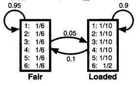
Our observations now are the values of the die roll. eg: 51245636664621212 and the hidden state that we are interested in is whether the die was loaded or fair eg: FFFFFLLLLLLLFFFFF.

Let's try generating a sequence of rolls given this model. On average how often do we expect the die to switch between states?

Are there specific subsequences where the Viterbi algorithm wouldn't work well? It's unlikely, but the casino could switch to the loaded die for a just one or two rolls. Do you think the Viterbi decoding would detect this switch?

From Chapter 3 of the Biological Sequence Analysis text we are given the example of changing our dishonest casino model so that npw the probability of staying fair is 99% rather than 95% with everything else staying the same. In simulations of this case, the Viterbi algorithm never visited the loaded state. In this case, the posterior decoding would have been a better approach (see page 59-61 in the chapter 3 of the text).