section 09: mixed feelings (k-means)
by Laila Norford and Jakob Heinz
k-means Live Simulation
Objectives
- Describe the steps of the (hard) k-means algorithm.
- Explain how the choice of initial centroids affects the final cluster assignments.
- Identify a solution to the problem of empty clusters.
- Determine how many clusters are appropriate for a given dataset.
Materials Needed
- 4 traffic cones / markers
- Tape or sidewalk chalk
- Tape measure
- Construction paper in four colors
Set-Up
- Measure and mark off a number line from -2 to 12. Put 2 feet between each number. Mark with tape or sidewalk chalk.
- Assign each student to an initial point:
6.54, 6.58, 0.02, 10.06, 10.14, 9.25, 3.33, 2.46, 6.35, 6.91, -0.23, 0.85, 9.27, 3.84, 10.28, 0.20
Activity
-
Begin by reviewing the steps of the hard k-means algorithm (initialization, assign points to nearest centroid to make clusters, update centroids, termination).
-
Have the students stand at their point on the number line.
-
Review methods to initialize k-means.
a. Choose K random points in space
b. Choose K random points from X and put the initial centroids there
c. Assign all points in X randomly to clusters, then calculate centroids of these
- 1st simulation (good initialization): -0.23, 0.20, 6.54, 9.27
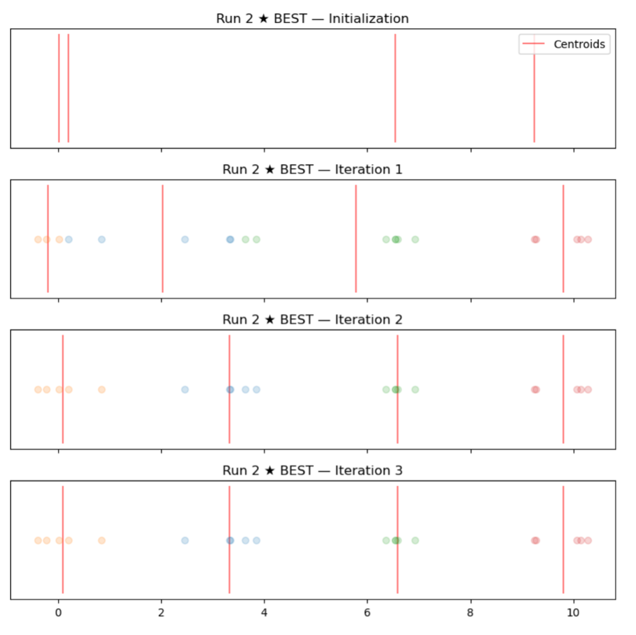
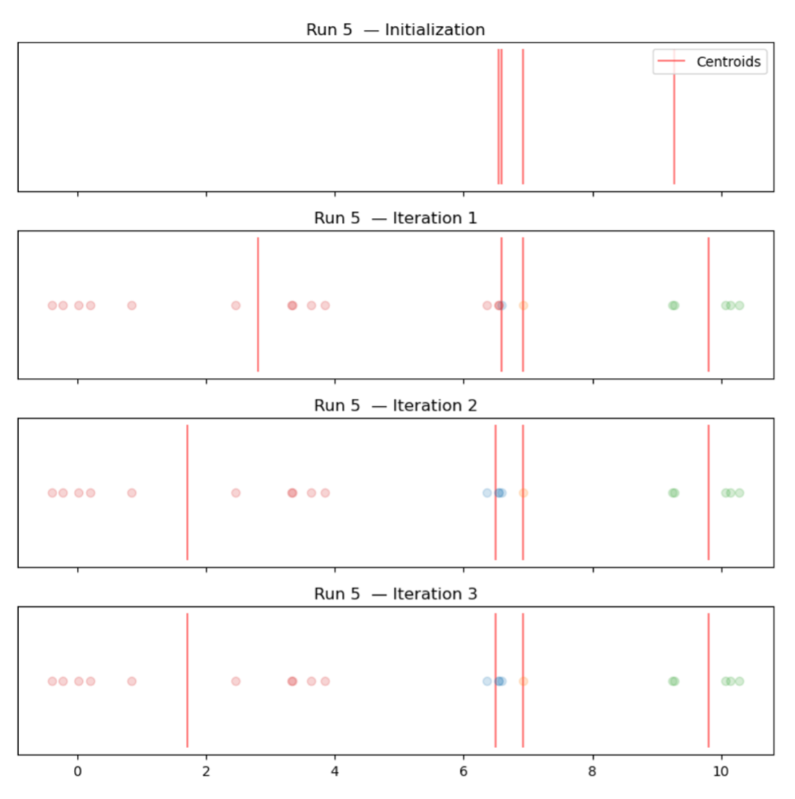
- 2nd simulation (bad initialization): 6.54, 6.58, 6.81, 9.27
- Discussion
a. Why we need to run the algorithm multiple times
b. How do we determine whether one run is better than another? (total distance)
- The empty cluster problem
a. Example initialization (choosing random points in space): 1, 4, 5, 6
b. 5 has no points assigned
c. Take the point farthest from its assigned centroid (10.28 will be farthest from its centroid, 6) and reassign the centroid to that point
d. Centroid at 5 Centroid at 10.28
- How do we know how many clusters?
a. In this case, I predetermined the clusters by manually selecting equidistant means and drawing from normal distributions at these means (with the same variance). Usually we won't know!
b. Elbow plot: you can try different values to see when you stop gaining information
- Adding more clusters beyond that point is overfitting
Coding k-means practice
Python notebook with examples [download] and solutions [download]