week 01: a fine playground for serious children
...the field of bacterial viruses is a fine playground for serious children who ask ambitious questions.
- Max Delbruck
Bacteriophages
We are going to concentrate MCB112 on genome sequence analysis problems, and specifically on problems involving bacteriophage (bacterial virus) genomes. One goal this week is to make sure everyone is up to speed on what a phage is, and what a phage genome sequence looks like.
how to isolate your own phage
Phage are everywhere, because bacteria are everywhere. There is an oft-cited estimate that there are about \(10^{31}\) phage on Earth.
What I'm doing here is called Fermi estimation. I only need to get a rough answer if I'm trying to judge if something is quantitatively plausible, biologically and/or physically. For the history of how people actually came up with the \(10^{31}\) estimate, see A. Mushegian, J Bacteriol, 2020. People like to pass along random unchecked statistics that sound impressive and quantitative, so we can and should quickly check how plausible a possibly-apocryphal number like this \(10^{31}\) phage number seems. The surface area of the planet is about \(2x10^8\) square miles (\(4 \pi r^2\), r=4000mi). If we assume that the phage biosphere is maybe 1-10 miles in height (from ocean floor to mountain peaks) and convert units to a phage titer in phage per milliliter, that means about \(10^6-10^7\) phage/ml on average, everywhere on Earth. Seems maybe a little high. But then again, it's easy to find data that in surface ocean water, there are typically about \(10^8\) phage per ml, so it's not likely to be super wrong, either.
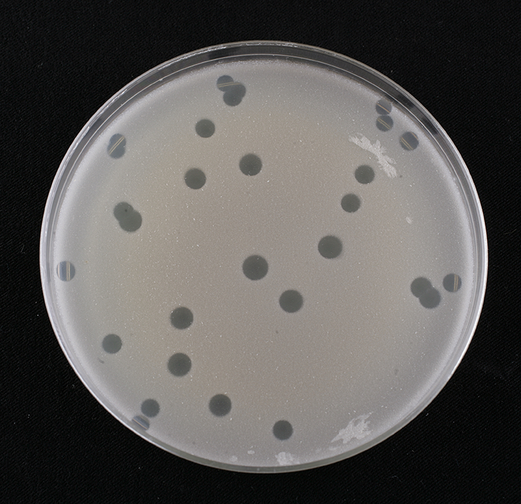 What phage plaques look like, on a lawn of their bacterial host. Each
hole in the lawn started as a single phage infection of one cell.
Source: SEA-PHAGES Discovery Guide.
What phage plaques look like, on a lawn of their bacterial host. Each
hole in the lawn started as a single phage infection of one cell.
Source: SEA-PHAGES Discovery Guide.
The abundance of phage means it's easy to find new ones. If you mix some bacteria (maybe E. coli) into some soft agar, pour it evenly over an agar plate, and let it grow overnight, you get a lawn, an even haze of bacterial growth over the plate. If you add an environmental sample to the bacteria and the soft agar, if the sample contains phage that can attack the host bacteria, you will get a visible plaque: a hole in the lawn where the phage replicated and killed all the bacteria in some radius. The radius depends on a number of factors including the growth rate of the phage and host, the "burst size" of the phage (how many new phage burst out of the cell in one complete growth cycle), and the size and diffusion rate of the phage in the agar.
You can then pluck one of those plaques with a pipette, and ta-da, you have your own new phage. Given how many phage there are on Earth, all evolving rapidly, it's very likely that no one has ever seen it before.
types of phage
Like all viruses, phage have a nucleic acid genome (DNA or RNA), packaged inside a protein capsid. They adsorb onto the surface of a bacterial host cell, inject their genome, and hijack the molecular biology of the cell to rapidly produce new phage genomes and structural proteins, package the genomes into new phage particles, and get out of the cell (often by lysing it). They depend on host functions for their replication, and are not free-living.
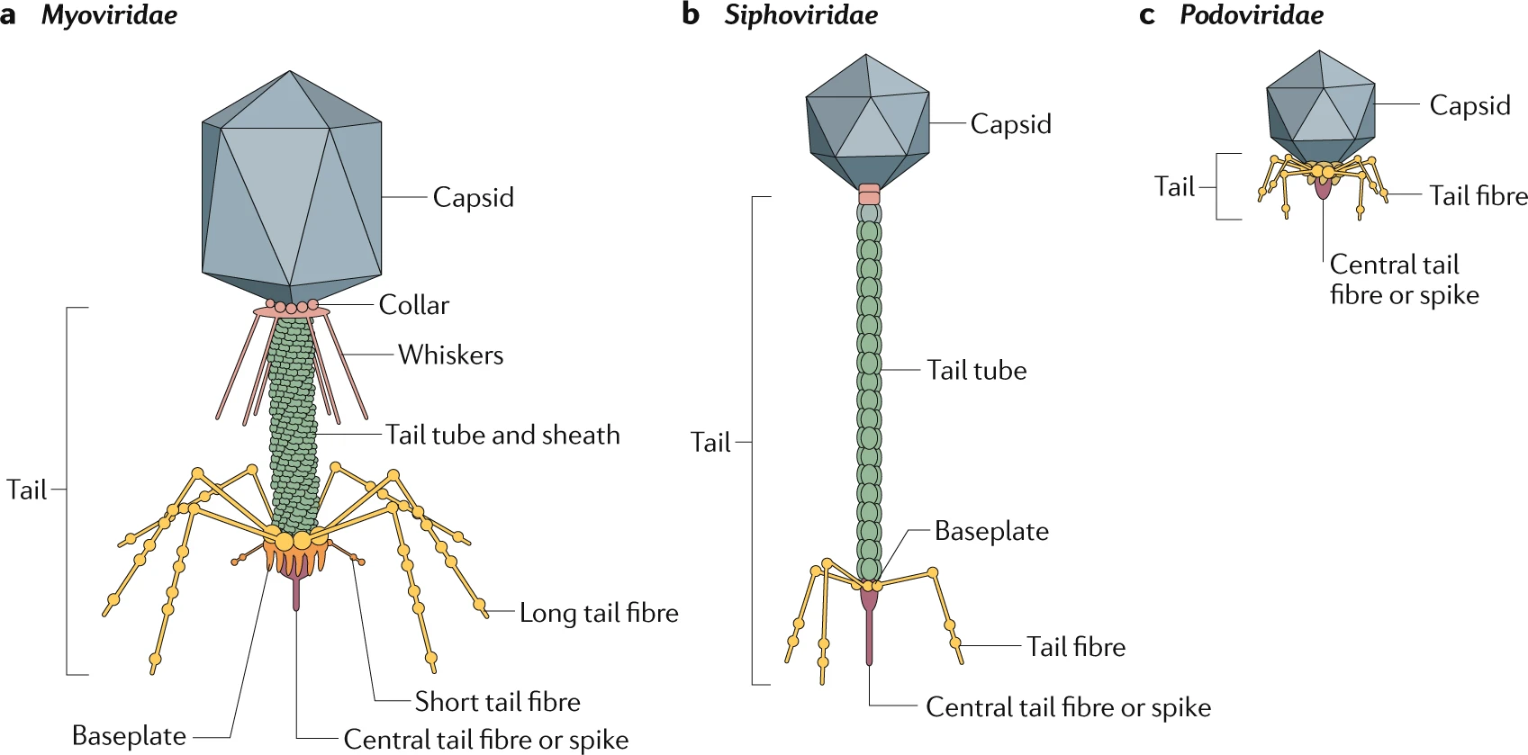 The most abundant phage are tailed double-stranded DNA (dsDNA) phage,
which come in three types: "Myoviridae" with long contractile tails
(including phage T4), "Siphoviridae" with long non-contractile tails
(including phage lambda), and "Podoviridae" with stumpy little tails
(including phage T7).
Source: Nobrega et al. (2018)
The most abundant phage are tailed double-stranded DNA (dsDNA) phage,
which come in three types: "Myoviridae" with long contractile tails
(including phage T4), "Siphoviridae" with long non-contractile tails
(including phage lambda), and "Podoviridae" with stumpy little tails
(including phage T7).
Source: Nobrega et al. (2018)
Phage come in many different kinds. The most abundant ones have double-stranded DNA (dsDNA) genomes. We'll talk a lot about one of these, one of the most famous and well-studied ones: phage T4, a Myovirus. Phage can also have single-stranded DNA genomes or RNA genomes; they can have tails or no tails.
Phage can be lytic: their life cycle destroys the host cell, emitting a burst of new phage. T4 is a good example of a lytic phage. Some phage are lysogenic: they quietly insert themselves into the host genome and go along for the ride for a while, expressing only a couple of their genes to keep an eye on how the host is doing; if the host is damaged or stressed, the phage activates a lytic cycle and escapes in a burst. Phage lambda is a good example of a lysogenic phage. When we analyze bacterial genome sequences, we find lysogenic phage genomes littered through them, some of which are still "alive" and intact, and others that are broken husks, decaying away in evolution.
Electron microscope image of phage T4.
Source: Miller et al (2003)
In the early days of molecular biology, there was a time when everyone was studying their own favorite phage isolate, and everyone was getting different results because there were so many different kinds of phage. In the American "phage school" that centered on Caltech and Cold Spring Harbor, Max Delbruck decreed that molecular biologists were only allowed to study one of seven phage ("Max's seven dwarves"), which were renamed type 1 through type 7: T1-T7. In Paris, quite a bit of work also focused on phage lambda. T2, T4, and T6 are similar to each other, T3 and T7 are similar to each other, T1 is weirdly dessication-resistant and thus capable of permanently contaminating laboratories, and T5 was unpopular for some reason - so over time people focused on T4, T7, and lambda as the main model systems for dsDNA phage.
| phage | genome | type | size |
|---|---|---|---|
| T1 | dsDNA | Siphoviridae | 50kb |
| T2 | dsDNA | Myoviridae | 170kb |
| T3 | dsDNA | Podovirus | 40kb |
| T4 | dsDNA | Myoviridae | 170kb |
| T5 | dsDNA | Siphovirus | 120kb |
| T6 | dsDNA | Myoviridae | 170kb |
| T7 | dsDNA | Podoviridae | 40kb |
| lambda | dsDNA | Siphoviridae | 50kb |
phage genetics
Phage T4 became particularly important to early molecular biology. If you ever want to know the answer to "what is a gene", start from classic T4 genetics.
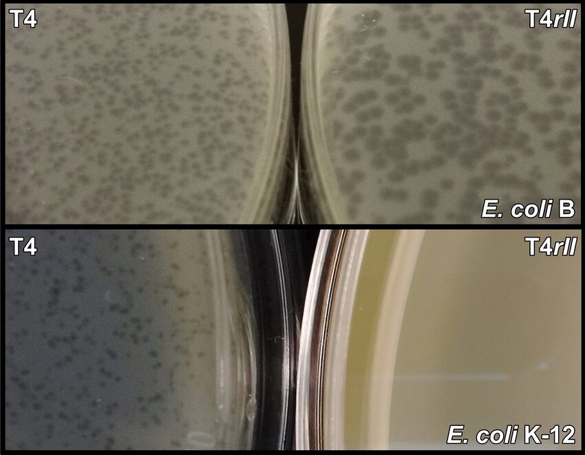 Plaque morphology
of T4 wild type phage (left) versus T4 rII mutant phage (right), on
a E. coli B strain host (top) versus an E. coli K12 strain host
(bottom). T4 rII mutants do not grow on K at all, but they do grow
on B, where they make abnormally large plaques.
Source: Wong et al. (2021)
Plaque morphology
of T4 wild type phage (left) versus T4 rII mutant phage (right), on
a E. coli B strain host (top) versus an E. coli K12 strain host
(bottom). T4 rII mutants do not grow on K at all, but they do grow
on B, where they make abnormally large plaques.
Source: Wong et al. (2021)
If you look at enough plaques, you can find mutants that have different plaque morphologies. You can also find mutants by screening for a successful plaque on a host or growth condition that the phage normally doesn't grow on, or if you're clever (with replica plates), phage that fail to grow on a host or growth condition they normally would.
One historically important genetic locus are is the T4 rII locus. rII mutants grow on E. coli B strains, but fail to grow on E. coli K strains. When they grow on B strains, they give large plaques. For geneticists, this is an unusual and advantageous situation: you can select for both rII+ phenotype and rII- phenotype, back and forth, by selecting rII+ phage that give plaques on a K lawn, and rII- phage that give large plaques on a B lawn.
Biologists at the time had no idea what a gene was (even whether it was DNA or protein), whether it was linear or branched or what, what the genetic code was, how proteins were encoded in a genome, or any of that. Simple experiments looking at whether T4 phage injects DNA or protein helped established that genes are DNA. With genetics and gorgeous logic, people established that genes were linear (by the fact that recombination maps of rII were linear), and that the genetic code is a triplet code (using an extraordinarily clever set of experiments combining frameshift mutations of rII).
A "gene", for example, was originally defined by genetic complementation tests. If you mix two mutants together at a high multiplicity of infection, so each cell is likely to get infected by both mutants, you are doing a complementation test. If the mutations are in different genes, then one mutant expresses one gene, the other mutant expresses the other, the infection succeeds, and you get wild type plaques. If the mutations are in the same gene, then neither mutant phage can express that gene, and you get mutant plaques. Complementation tests on rII mutants showed that there were two rII genes, rIIA and rIIB.
One important class of mutants were called "amber" mutants. Many different genes were found that all had the property of not growing on a E. coli B host, but growing well on a particular E. coli K host. Because this was such a general class of mutants, people could rapidly catalog and number genes in T4. To this day, many T4 genes are identified by their number; gene 43 is the DNA polymerase, gene 23 is the major capsid protein, and so on. It turned out, much later, that that K host is expressing a suppressor tRNA that reads TAG stop codons as a sense amino acid, and the T4 amber mutants are all cases of creating a TAG stop codon in the middle of a gene's coding region.
the SEA-PHAGES undergraduate courses
An HHMI-sponsored undergraduate lab course called SEA-PHAGES (Science Education Alliance - Phage Hunters Advancing Genomics and Evolutionary Science) runs at several colleges across the US. Students in the course isolate their own new phage from soil, name it, and sequence and annotate its genome.
The SEA-PHAGES project has a nice Discovery Guide about how their phage discovery works, including a good introduction to phages.
I have a dataset of about 5000 SEA-PHAGE genome sequences that we will focus on for many of our problem sets. I'll supplement that sometimes with additional phage datasets, when the SEA-PHAGE don't suffice for my purpose.
a closer look at phage T4's structure and genome map
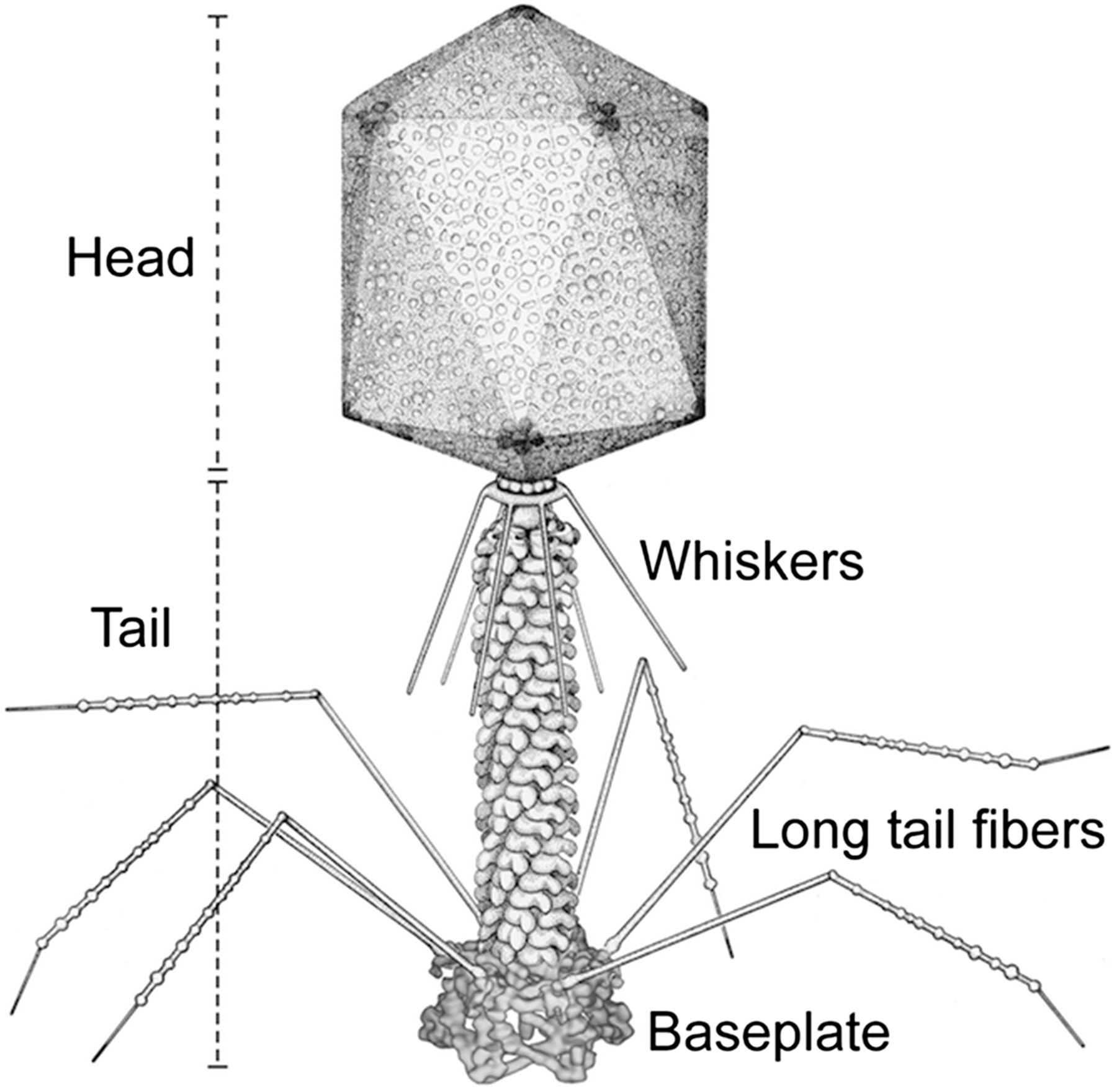 The structure of bacteriophage T4.
Source: Yap et al (2016).
The structure of bacteriophage T4.
Source: Yap et al (2016).
T4 is a complex phage, with a genome of about 170kb, encoding about 300 different protein-coding genes. The genome was originally mapped by genetics.
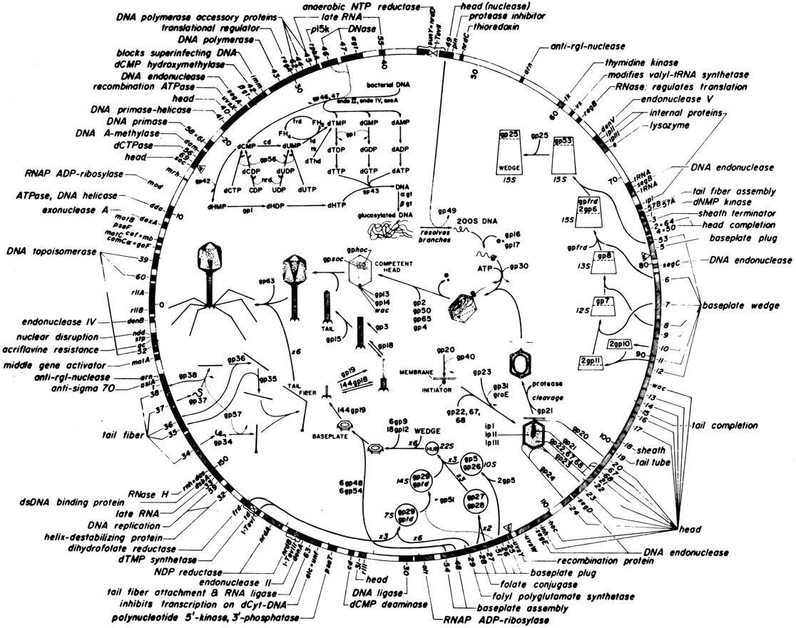 The circular genetic map of the linear phage T4 genome.
Source: Sulakvelidze et al (2001)
The circular genetic map of the linear phage T4 genome.
Source: Sulakvelidze et al (2001)
When T4 replicates its DNA, it makes a very long concatenated product, which is then packaged by a "head-full" mechanism: it packages as much DNA as will fit, which is about 172kb, just slightly more than one 169kb genome, so there is a terminal redundancy of a few kilobases. Each packaged individual phage has a different terminal redundancy, which produces a curious genetic effect: the genetic map of phage T4 is circular, even though the genome is physically linear.
A more modern genome map of phage T4, showing the annotated genes.
Source: Miller et al (2003)
The 169kb T4 genome was sequenced in the 1980's and 1990's, and its 300 or so known genes were annotated on that sequence. (Which we'll dive into soon.) The protein-coding genes are the dominant feature of the genome. Phage genomes are compact and gene-dense. The genome sequence is almost 100% covered by annotated genes.
Many of these genes make the structural proteins of the capsid, tail, baseplate, and tail fibers, which self-assemble (even in a test tube) to produce phage particles. This makes sense: during infection, it will make about 100-200 new phage particles, so these new structural proteins plus 100-200 new genomes is the ultimate goal for the phage.
To replicate its DNA, T4 encodes genes for its own replication and recombination machinery, including the gene 43 DNA polymerase.
The demand for DNA nucleotides is about 10-fold higher than the host cell can support. 100-200 phage genomes in a 30' lytic cycle means about 30Mb of new DNA, whereas E. coli would normally be making one new 4Mb genome in that time span. Therefore T4 also brings in a set of genes for its own nucleotide synthesis machinery, to convert ribonucleotides to deoxyribonucleotides.
There's another 20 phage-equivalents of deoxynucleotides in the host genome itself, and the host won't be needing it now that it's dead, so T4 expresses genes to degrade and digest the host genome down to single dNMPs, and kinases them up to dNTPs.
To transcribe its genes as mRNAs, T4 does not make its own RNA polymerase; it steals and modifies the host RNA polymerase to make it more and more specific for T4 genes. "Early" genes have promoters that look like host promoters. "Late" genes have promoters with a different upstream consensus sequence, because T4 replaces the normal E. coli RNA polymerase specificity subunit (the "sigma factor") with a phage-specific one, the product of gene 55.
A defining feature of viruses (so far) is that viruses do not produce their own ribosomes; they use the host ribosomes. T4 has some proteins that put modifications onto E. coli ribosomes for purposes that I think still remain unclear.
These categories of genes - structural proteins, replication and recombination, nucleotide synthesis, transcriptional and translational regulation - all make logical sense, from a design-your-own-phage-in-your-basement perspective. But they only account for about half of T4's genes.
The other half appears to consist of molecular weaponry, in a battle between the phage, the host, and other phages. The host bacterial genome expresses restriction enzymes to target and cut up phage DNA as it's injected; the phage modifies its DNA to make it resistant to restriction. The host expresses adaptive CRISPR systems to destroy the phage; the phage makes anti-CRISPR systems. The host makes suicide mechanisms ("abortive infection" systems) that detect an infection in progress and the cell kills itself to protect its brethren. The complexity and cleverness of these systems is amazing, and still being worked out. It's been a source of many of the best tools in molecular biology, including restriction enzymes in the olden times, and CRISPR most recently.
The T4 rII genes appear to be involved in some sort of weapons/counterweapons dance with phage lambda, for example. The K12 strain that restricts rII mutants turned out to be a lambda lysogen. Along with the famous lambda repressor that any molecular biology class or textbook tells you about, phage lambda lysogens also expresses two other less well known genes called rexA and rexB which appear to form a suicide switch of some sort: when T4 rII mutants infect a lambda lysogen, rexA and rexB form an ion channel that collapses the proton gradient that is needed for ATP generation, and the cell dies. The rII genes appear to be some sort of counterweapon against rex. How this system actually works in detail remains unknown.
the T4 genome sequence
The best way to get started with genome sequence analysis is to look at a genome, especially one that makes sense. Here's the T4 genome, as a GenBank file. You can also obtain it from NCBI GenBank itself.
The top of the file tells us what we're dealing with:
LOCUS       NC_000866             168903 bp    DNA     linear   PHG 11-JAN-2023
DEFINITION  Enterobacteria phage T4, complete genome.
ACCESSION   NC_000866
VERSION     NC_000866.4
DBLINK      BioProject: PRJNA485481
KEYWORDS    RefSeq.
SOURCE      Escherichia phage T4
  ORGANISM  Escherichia phage T4
            Viruses; Duplodnaviria; Heunggongvirae; Uroviricota;
            Caudoviricetes; Straboviridae; Tevenvirinae; Tequatrovirus;
            Tequatrovirus T4.
There's so many viruses that in viral phylogenies, the taxonomists sometimes sort of throw up their hands with the nomenclature. "Tequatrovirus" is a pretty lazy name for the genus that includes T4.
Then there's a long list of references that you can skip past. Many GenBank entries are from a single paper, but the T4 genome sequence was a community effort over many years and papers, so there's an unusual number of sources cited. Skip down to where the FEATURES section starts. Oh look! the first gene, by convention, is rIIA:
  gene            complement(12..2189)
                     /gene="rIIA"
                     /locus_tag="T4p001"
                     /db_xref="GeneID:1258593"
     CDS             complement(12..2189)
                     /gene="rIIA"
                     /locus_tag="T4p001"
                     /note="membrane integrity protector; mutants give rapid
                     lysis on various lysogenic strains due to effects of
                     specific prophage products, mistakenly interpreted as
                     related to lysis inhibition"
                     /codon_start=1
                     /transl_table=11
                     /product="RIIA lysis inhibitor"
                     /protein_id="NP_049616.1"
                     /db_xref="GeneID:1258593"
                     /translation="MIITTEKETILGNGSKSKAFSITASPKVFKILSSDLYTNKIRAV
                     VRELITNMIDAHALNGNPEKFIIQVPGRLDPRFVCRDFGPGMSDFDIQGDDNSPGLYN
                     SYFSSSKAESNDFIGGFGLGSKSPFSYTDTFSITSYHKGEIRGYVAYMDGDGPQIKPT
                     FVKEMGPDDKTGIEIVVPVEEKDFRNFAYEVSYIMRPFKDLAIINGLDREIDYFPDFD
                     DYYGVNPERYWPDRGGLYAIYGGIVYPIDGVIRDRNWLSIRNEVNYIKFPMGSLDIAP
                     SREALSLDDRTRKNIIERVKELSEKAFNEDVKRFKESTSPRHTYRELMKMGYSARDYM
                     ISNSVKFTTKNLSYKKMQSMFEPDSKLCNAGVVYEVNLDPRLKRIKQSHETSAVASSY
                     RLFGINTTKINIVIDNIKNRVNIVRGLARALDDSEFNNTLNIHHNERLLFINPEVESQ
                     IDLLPDIMAMFESDEVNIHYLSEIEALVKSYIPKVVKSKAPRPKAATAFKFEIKDGRW
                     EKRNYLRLTSEADEITGYVAYMHRSDIFSMDGTTSLCHPSMNILIRMANLIGINEFYV
                     IRPLLQKKVKELGQCQCIFEALRDLYVDAFDDVDYDKYVGYSSSAKRYIDKIIKYPEL
                     DFMMKYFSIDEVSEEYTRLANMVSSLQGVYFNGGKDTIGHDIWTVTNLFDVLSNNASK
                     NSDKMVAEFTKKFRIVSDFIGYRNSLSDDEVSQIAKTMKALAA"
This says that the rIIA gene (from start codon to stop codon, inclusive) runs from position 2189 to position 12 on the reverse strand, where the coord system is 1..L for L=168903. So that means it encodes 725 sense triplets (ending with one stop triplet), encoding a 725 amino acid protein. If we extract coords 2189..12, that looks like:
>NC_000866/2189-12 NC_000866.4 Enterobacteria phage T4, complete genome.
atgattatcaccactgaaaaagaaacaattcttggtaatggttctaaatcaaaagcattt
agcatcacagcatctcctaaagtatttaaaattctgtcatctgatttgtatacaaacaag
... lots more nucleotides ...
ttcatcggttatcgcaactctttaagtgatgatgaagtttcccaaatcgctaaaactatg
aaggcccttgcggcctaa
and we can see the ATG start codon and a TAA stop codon.
The spaces in between the genes are where there are regulatory sequences for controlling the transcription and translation of the gene. The upstream gene is rIIA.1 from 2043..2200 (also on the opposite strand), so the intergenic sequence between rIIA.1 and rIIA is 2199..2190, just 10 nucleotides:
tgaggaaatt
And in this, by eye, I can see a regulatory sequence called the Shine/Dalgarno (S/D) consensus. Bacterial ribosomes initiate internally on an mRNA by recognizing a ribosome binding site (RBS): a start codon with a short S/D consensus sequence a few bases upstream. The 3' end of the ribosomal RNA is complementary to the S/D. The S/D consensus is UAAGGAGGA, where any 4- or 5-nt substring centered around the G's is typical: GGAGG, GAGG, AGGA, etc. And looky there: GAGGA, then a 4 nt spacer, then the rIIA ATG. A classic Shine/Dalgarno ribosome initiation site.
Phage genomes are so densely packed that intergenic spaces are small, and regulatory sequences are typically easy to analyze and find. We will take thorough advantage of that in the course.
Browse through the rest of the feature table -- most of it is the annotated 300 or so genes. Skip down to a line that starts with ORIGIN:
     gene            complement(167965..168903)
                     /gene="rIIB"
                     /locus_tag="T4p278"
                     /db_xref="GeneID:1258618"
     CDS             complement(167965..168903)
                     /gene="rIIB"
                     /locus_tag="T4p278"
                     /note="membrane integrity protector; mutants give rapid
                     lysis on various lysogenic strains due to effects of
                     specific prophage products, mistakenly interpreted as
                     related to lysis inhibition"
                     /codon_start=1
                     /transl_table=11
                     /product="RIIB lysis inhibitor"
                     /protein_id="NP_049889.1"
                     /db_xref="GeneID:1258618"
                     /translation="MYNIKCLTKNEQAEIVKLYSSGNYTQQELADWQGVSVDTIRRVL
                     KNAEEAKRPKVTISGDITVKVNSDAVIAPVAKSDIIWNASKKFISITVDGVTYNATPN
                     THSNFQEILNLLVADKLEEAAQKINVRRAVEKYISGDVRIEGGSLFYQNIELRSGLVD
                     RILDSMEKGENFEFYFPFLENLLENPSQKAVSRLFDFLVANDIEITEDGYFYAWKVVR
                     SNYFDCHSNTFDNSPGKVVKMPRTRVNDDDTQTCSRGLHVCSKSYIRHFGSSTSRVVK
                     VKVHPRDVVSIPIDYNDAKMRTCQYEVVEDVTEQFK"
ORIGIN
        1 aattttcctt attaggccgc aagggccttc atagttttag cgatttggga aacttcatca
       61 tcacttaaag agttgcgata accgatgaag tcggaaacaa tacggaattt cttggtaaac
      121 tcagcaacca ttttatcact gttttttgaa gcattatttg ataatacatc aaaaagatta
[... lots of nucleotides ...]
   168781 acggattgtg tcaaccgata caccttgcca atcagccaat tcctgttggg tgtaattacc
   168841 acttgaatac agtttaacaa tttcagcttg ttcgtttttg gtcaggcatt taatattgta
   168901 cat
//
and after the traditional arbitrary "last gene" rIIB on the circular genetic map, we get the actual 168903nt sequence, in lines of 60 nucleotides with a leading coordinate. If you were writing a parser to get a DNA sequence from a GenBank file, you'd focus on the bit between the ORIGIN and the terminating "//" line, and you'd skip the numbers and the whitespace.
world's fastest intro to molecular biology
With the actual T4 genome sequence in mind (specifically: it's pretty much all coding region, there's not much room for regulatory sequence), let's now review the central dogma:
A gene is transcribed to an mRNA copy. The RNA polymerase recognizes and binds a consensus promoter sequence upstream of the mRNA start site. In E. coli, the standard \(\sigma^{70}\) promoter consensus consists of two pieces, one at roughly -35 from the start site (TTGACA) and one at roughly -10 (TATaaT). T4 late genes are expressed from a different promoter consensus. By recognizing RNA polymerase promoter site sequences, we can predict the start site of each mRNA.
Transcription continues until the polymerase reaches a terminator. Bacteria (and their phage) have two types of terminators: rho-independent terminators that are pretty easy to recognize (the consensus is an RNA stem-loop followed by a run of T's), and rho-dependent terminators (that depend on a protein termination factor called \(\rho\)) that are not actually all that predictable or understood yet.
Genes are turned on and off often at the level of controlling mRNA expression, using DNA-binding proteins that repress or activate transcription. These DNA-binding proteins typically bind near the promoter to either block polymerase from its site (thus repressing transcription), or nestling adjacent to it and doing something to activate it. One particular famous example is the lac operon repressor, and another is the lambda repressor that controls phage lamba's lytic/lysogenic switch. Transcriptional regulatory DNA-binding proteins have consensus recognition sites that we can computationally infer in genome sequence.
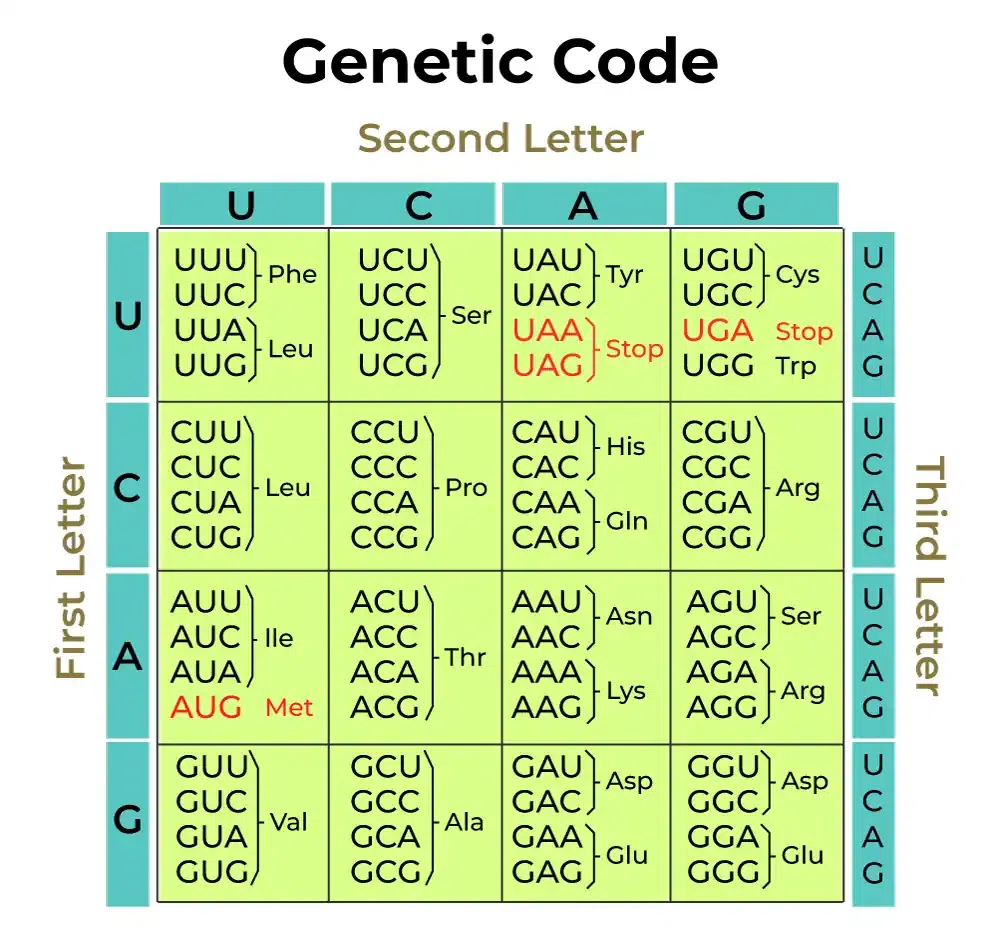 The standard genetic code.
Source
The standard genetic code.
Source
In bacteria and phage, one mRNA transcript often spans several genes in a row and encodes separate proteins from them: bacterial genes are organized in operons. A famous example is the lac operon of E. coli, which makes one mRNA transcript that encodes four genes for lactose usage - lacI, lacZ, lacY, and lacA. lacY is a permease that transports lactose into the cell. lacZ is \(\beta\)-galactosidase, which digests the lactose disaccharide into galactose and glucose. lacA is a transacetylase whose role remains murky even today. lacI is the lac repressor, which binds to an operator in the lac promoter to keep the operon off unless lactose is present. Operon structure is an important clue to the genome sequence analyst: if you know the function of some genes in an operon, you can bet that the rest of the genes function in the same pathway or process, such that they're all being turned on and off at the same time by transcriptional regulation.
An mRNA is then translated to protein(s). The ribosome binds to an internal ribosome binding site (already mentioned) to define the start codon for a coding region. The ribosome then reads three nucleotides at a time (codons) and, following the rules of the genetic code, translates each codon into an amino acid that's added to a growing polypeptide chain, using adaptor molecules called transfer RNAs (tRNAs) that have a complementary anticodon at one end, and the amino acid to add at the other. Translation stops when the ribosome reaches a stop codon: TAA, TAG, or TGA.
The standard genetic code is almost but not quite universal. Human mitochondria, for example, read TGA as Trp, ATA as Met, and don't read AGA|AGG at all. Some phage actually change the genetic code during infection, using the host code in early gene expression, and switching to recoding the TAG or TGA stop codon for late gene expression. The non-universality of the genetic code is the topic of the pset this week!
Not all genes encode proteins. Ribosomes are mostly RNA-based machines, dominated by ribosomal RNA (rRNA), and the transfer RNAs that ribosomes use to decode triplets in mRNA are RNAs. Ribosomes are so abundant in cells that most of the RNA in a cell is rRNA - functional RNA - not mRNAs coding for protein. This jammed people up for a long time. How does information get from DNA sequence to protein sequence? If RNA is the intermediary, then there should be a different RNA for every gene, but biochemists had clearly observed with the crude methods of the time that the majority of RNA in a cell was all the same sequence (i.e. rRNA). Then someone did an experiment showing that after T4 infection, almost all the RNA in the cell stayed the same (again, because it's rRNA, and T4 is using the host ribosomes) but a new, minority fraction of RNA appeared that had the same AT-rich composition as the T4 genome. The light immediately dawned - that tiny fraction of unstable RNA is mRNA, against a massive background of the ribosomal RNA machines.
There are whole textbooks on molecular biology, of course (and you should read at least one of them).
For MCB112, a great thing about phage genomes (as opposed to horrible junk-ridden mammalian genomes) is that phage genomes make sense. They are packed with information. mRNA transcription units, coding regions, regulatory DNA and RNA binding sites are readily and intuitively predicted from a single genome sequence and/or genome sequence comparisons. We can read these genomes almost like a book. They're a great place to learn a whole bunch of stuff about computational molecular biology.
Practicalities
GenBank and FASTA sequence file formats
During the course, we will see sequence files in two standard formats.
One is GenBank format, like the T4 genome file above. GenBank format allows for extensive annotation of features and references. When you sequence a new phage genome, you would typicaly deposit your genome sequence and annotation with NCBI and it goes into GenBank (which then shares it with international collaborators, the DNA Database of Japan, DDBJ, and the European Nucleotide Archive, ENA).
The other is FASTA format. FASTA is a simple and widely used lowest-common-denominator format for DNA, RNA, and protein sequences. Like many bioinformatics formats, it is flexible but poorly standardized; so much so that different documentation on FASTA format is typically inconsistent in subtle ways. The features you can rely on are as follows.
Each sequence has a header line that starts with >, followed by the
sequence name (one "word", whitespace-delimited). The remainder of
the header line is an optional free-text description. To be
maximally safe, don't put any space between the > and the name; some
programs won't recognize the name if you do.
Lines after the header lines are the sequence. To be maximally
safe as a FASTA input file, these lines should be short (60-80
character lengths are typical), and contain nothing but legal IUPAC
one-letter sequence codes for DNA or protein. It's generally not safe
to use the RNA U instead of DNA T, because many programs won't
recognize that U and T are the same, or may not recognize U at all.
An example:
   >NM_001168316  Description of sequence one.
   TTAGTGAGGTTGGGGAGAGATAACGCTGTAAACTTTTATTTTTCAGGAAATCTGGAAACC
   TACAGTCTCCAAGCCTGCTCAGCCAAGAAGGAGCTCACTGTGGGCACCAGAGACAGGGAC
   CATTT
   >NM_174914 Description of sequence two.
   TTAGTGAGGTTGGGGAGAGATAACGCTGTAAACTTTTATTTTTCAGGAAATCTGGAAACC
   TACAGTCTCCAAGCCTGCTCAGCCAAGAAGGAGCTCACTGTGGGCACCAGAGACAGGGAC
   CCAATGTGGAGACCTGTGAGCCTGTGTCCGGCCCTGAA
sequence residue character codes, DNA and protein
The four bases of DNA are abbreviated A,C,G,T. In RNA, uracil replaces thymine, so you may see U characters in RNA sequence files.
The 20 amino acids are abbreviated ACDEFGHIKLMNPQRSTVWY. It's worth memorizing these one letter codes.
In MCB112, you will usually be able to assume that all characters (which I'll often call "residues") are the canonical 4 or 20 for DNA or protein. But in real data, be aware that there are a host of other one letter codes in use, to represent either ambiguities in sequencing, or real biological modifications. For example, for DNA sequence, N means any base A|C|G|T; R means purine A|G; and many more. For protein, X means any amino acid, B means Asp|Asn, Z means Glu|Gln, J means Ile|Leu, U means selenocysteine, and O means pyrrolysine. B and Z are there because old-school protein sequencing (by Edman degradation) could not distinguish D|N or E|Q. J is there because new-school protein sequencing (by mass spec) can't distinguish I|L. U and O are there because even though everyone told you there are 20 genetically-encoded amino acids, actually there's 22 (so far). (The other two known genetically-encoded amino acids are selenocysteine and pyrollysine.)
The most important additional codes are controlled formally by an international committee, IUPAC. Other codes are in use out there for specialized purposes - for example, people will make up a way they like to represent modified RNA bases in RNA sequence files. Watch out.
Conversely, just because a sequence file says a base is A, C, G, or T, doesn't mean it is -- various organisms put all sorts of modifications on their DNA (and RNA) for a range of important biological purposes, and our sequencing technologies (and sequence file formats) are not always able to detect or represent these modifications. In human DNA, a famous one is CpG methylation, where C's are converted to 5'-methylcytosine at CpG dinucleotides; we saw this mentioned in pset w00. Phage T4 has a spectacular one: to protect itself against the host trying to kill it by targeting and degrading its DNA with restriction enzymes, T4 converts essentially all its C's to 5'-hydroxymethylcytosine, and then for good measure it glycosylates (adds a sugar to) the 5'hmC modification, with the result that it basically fills its DNA major groove with sugar, keeping host restriction enzymes from probing its DNA sequence.
basic Python... but with a little NumPy this week
In each pset, I will specify what Python modules you're allowed to use. This is to limit the complexity of the Python code you write for the class -- partly so we have a simplified on-ramp for people who've never coded before, partly to concentrate on fundamentals and avoid black box solutions, and partly to make it easier for us to grade.
A standard Python installation comes with over 200 built-in modules, not to mention thousands of other third-party modules available in the Python ecosystem (including NumPy, matplotlib, Pandas, SciPy). We're going to use as few of them as possible in the course.
This week the pset would be all basic Python (i.e. no module imports)
except for one thing: random number generation, which you can do
either with the standard random module, or with NumPy
np.random().
You might also find yourself doing some math, and some basic math
functions like log() and exp() are both in the standard math
module and in NumPy.
Here I'll introduce just a smidgen of NumPy for both things. The heart of NumPy is elsewhere, in how it enables you to compute on arrays (and vectors, and tensors) of numerical data, and we'll delve into that next week when we introduce NumPy for real.
random numbers
To simulate data sets, we need to do random
sampling. The
most basic routine is a random number generator (RNG) that generates
a uniformly distributed sample on some interval. It's very common for
RNGs to provide a floating point value \(u\), uniformly distributed on
the interval \(0 \leq u < 1\): \(u\) can be exactly zero, but it isn't
exactly one. This is what NumPy provides: There
are often many ways to do things in Python. We can also use the
random module from the Python standard library, and even within
NumPy, there is another way to generate random numbers using
np.random.*() functions. My style is to figure out one good way that
works for me, put it in my notes (I have a big "cheat sheet" of Python
notes that I refer to when I'm coding), and stick with it. The way I'm
showing you here is the current recommended way to do things in NumPy.
   rng = np.random.default_rng()  # Create an RNG
   u   = rng.random()             # Sample a single random number on [0,1)
   V   = rng.random(10)           # Sample a vector of 10 random numbers
   A   = rng.random((2,10))       # Sample a 2x10 array of random numbers
Note that rng is an object that we create (specifically, a
Generator object), and random() is a method in the Generator.
There's a lot to say about random number generators, but two of them are super important.
The first thing is that almost all random number generators (RNGs; including the "Mersenne Twister" generator that NumPy uses) are actually pseudorandom. The sequence of numbers they generate appears statistically random, but if you start the generator in the same internal state, you get exactly the same sequence.
Because cryptography algorithms often depend on random number generation, cryptography aficionados go all haywire about pseudorandomness. If you know the RNG algorithm and you can deduce its internal state, you can completely predict everything the RNG will generate. This is less than optimal, as you can imagine, if that sequence was supposed to be a secret.
The internal state of an RNG is initialized by a single number called the seed. If you initialize the RNG with the same seed, it generates a reproducible sequence of numbers. You can try that in NumPy for yourself:
   rng = np.random.default_rng(42)   # '42' is the seed
   for i in range(10):
      print(rng.random())
Execute that code (or Jupyter notebook cell) several times; you'll see the same sequence of "random" numbers.
Which brings us to the second thing. Sometimes you want to get a reproducible result from your simulation experiment, but sometimes you want to run independent replicates. If you want a reproducible result, you run with a fixed RNG seed. If you want independent replicates, you run each replicate with a different RNG seed.
If you don't provide a seed when you create the RNG with
np.random.default_rng(), the RNG will be created with a random seed,
so it generates a different stream of numbers each time you run your
program or Jupyter cell.
A bit of a chicken and egg problem - does NumPy use an RNG to get a
random seed to make an RNG? np.random.default_rng() does some black
magic to "pull entropy" from the operating system to obtain a random
seed. Be aware that there are many ways that code might try to
generate a pseudorandom seed, and many of them are bad. You may
encounter their shortcomings. For example, you may someday encounter
code that internally uses the system clock time to generate a "random"
seed, and clock time on some systems might be in units of seconds. Thus, if you start
many instances of your program quickly (like, firing off 100 replicate
runs from a script), ones that start in the same time interval will
get the same RNG seed and produce identical results. This is not what
you want. Yes, this has happened to me.
random sampling
On the sturdy back of uniform [0,1) sampling with random(), NumPy
then builds a large variety of random sampling
methods.
Some of the most useful ones for us to start with include:
n = rng.integers(1,7)                             # Choose uniformly distributed random integer from 1 to 6 (yes, 6; [low,high) half-open interval)
V = rng.integers(1,7,10)                          #  ... a vector of 10 die rolls
A = rng.integers(1,7, (4,10))                     #  ... an array of 4 rows of 10 die rolls

n = rng.integers(low=1, high=7)                   # Same as above, but using keyword args, which can make things more self-documented
V = rng.integers(low=1, high=7, size=10)          #
A = rng.integers(low=1, high=7, size=(4,10))      #

c = rng.choice(list('ACGT'))                      # Choose random element from a list uniformly; here, ['A','C','G','T']
c = rng.choice(list('ACGT'), p=[0.1,0.1,0.7,0.1]) # Choose random character nonuniformly with specified probabilities

A = rng.choice(list('ACGT'), size=10 0)           # Choose an array of 100 random ACGT's
S = ''.join(rng.choice(list('ACGT'), 100))        # a string's `join` method concatenates list/array onto its end; you can make a string from a list

u = rng.normal(mean, stdev)                       # Sample from a Gaussian (assumes you've set the `mean` and `stdev` variables, of course)

A = list('ABCDEFGHIJ')
rng.shuffle(A)                                    # Shuffle a list or array in place
manipulating and transforming strings
Data types in Python are objects, and objects have methods that you can call on them to manipulate their contents. Even things that seem like bedrock-basic data types, like an integer, are objects with methods. You get used to this. (I'm a C programmer, so for me, it takes a lot of getting used to.) A good and useful place to practice Python's style of calling methods on objects is with strings. It will be natural in this week's pset to store and manipulate DNA sequences as strings.
Here's some starting examples:
    S  = '{:.2f}'.format(1.2345)           # S = '1.23'
    S  = ','.join(['abc', 'def', 'ghi'])   # S = 'abc,def,ghi' (concat a list, with <str> as the separator!)
    S  = 'acgt'.upper()                    # S = 'ACGT'
You will use
<str>.format()
method a lot in print statements. It lets you insert and format your
variables for printing. The most basic way to use it is something like
print('my value = {}'.format(x)'. The format method looks for the
{} in the string, and replaces it with the value of x.
Another (more compact and more recent) way to do this is with what Python
calls "f-strings": print(f'my value = {x}').)
With more than one {} in the string, format() will replace them
with the corresponding value from its argument list, in
order: print('x = {}, y = {}'.format(x,y)).
If you include a number inside the {}, you can reorder (or repeat)
values from the argument list: print('y = {1}, x =
{0}'.format(x,y)).
If you include a : (after the optional number), format will
interpret what comes next as a compact instruction for how to format
the value it prints. For example, you only want to print floating
point numbers to a reasonable number of significant digits;
print('x = {.2f}'.format(x)) says that x is a float (that's the f)
and to print it with a precision of two digits after the decimal point
(that's the .2).
Learn how this formatting works by trying it out in a notebook cell, while consulting a tutorial or the documentation.
The .join() method is a little arcane: this is a way (arguably the
best way) to convert a list into a string. If I have a DNA sequence
as a list L = [ 'A', 'C', 'G', 'T' ], and I want to convert it to a
string S = 'ACGT', I call S = ''.join(L). If I want to convert
the string back to a list, I call the more intuitive L = list(S).
There are a gazillion other string methods you can call. In the
example above, <str>.upper() converts all lower-case characters to
upper-case. Again, the best way to learn them is playing with them in
a notebook cell, while consulting
documentation.
Here's a more complex example that will be useful in this week's
homework (though there are a jillion other ways to do this
too). <str>.translate(tbl) translates each character in <str> to
another character, according to a so-called "translation table"
<tbl>. You create a translation table using str.maketrans(from,
to), where (a detail!) str is literal, not a variable
(str.maketrans is a so-called static method). For example, this
little useful incantation:
S = 'AAAAAAAAAAAAAA'.translate(str.maketrans('ACGT', 'TGCA'))
returns 'TTTTTTTTTTTTTT', having converted A's to T's (and C to G, G to C, T to A). Guess where in the pset you might want to use that.
further reading
The Eighth Day of Creation, Horace Freeland Judson, manages to tell the history of molecular biology in a way that reads like a novel while being accurate in the science.