week 03: data exploration and visualization
The term "data science" seems to have been introduced in its current sense by W. S. Cleveland in 2001. W.S. Cleveland, Data science: an action plan for expanding the technical areas of the field of statistics, International Statistical Review, 2001. David Donoho's 50 years of data science is an excellent summary of what "data science" means, especially from the perspective of how academic disciplines are organized, how they change over time, and how statistics departments didn't see this coming.
Donoho repeats a famous quote that 80% of the effort in data analysis is just being able to deal with the messiness of real data: reformatting, exploring, cleaning, visualizing. In biology, 80% is an understatement.
This week, we're going to focus on some of the data science aspects of biology - with a particular focus on manipulating 2D tabular data files.
a data paranoia toolkit
The first thing you do with a new data file is look at it. But, you say, come on, my file is too big to read the whole thing. Pshaw. Here's a litany of basic techniques for dealing with big data files, aiming to get unmanageably big data sets down to little data sets that you can put your intuitive human eyes on:
- slice: look at the start and the end
- select: look at known cases
- sample: look at a random sample
- sort: look for outliers
- summarize: look for more outliers
- validate: the whole file, once you think you understand it.
We'll focus here on simple line-oriented data files (like tabular data), but the same ideas apply to more complex data types too.
I'll also use this as a stealth intro to some of the power of your command line and unix-y command line utilities. This week we also introduce the Pandas data science environment for Python. Part of your work on the pset will be using Pandas methods for similar things.
look at the start, end
The best place to start is at the beginning. The start of the file tends to include helpful information like column headers, comments, and other documentation. If you're going to parse the file, this might help -- plus your parser might have to know to skip or specially deal with header material.
To look at the start of a file on the command line:
% head -10 Moriarty_SuppTable1.tsv
shows you the first 10 lines of the file. (Obviously, you can use this to get however many you want to read.)
Worth checking the tail end of the file too. It might end in a special kind of line that you'd need to parse. A corrupted file (in a truncated download) might end abruptly in an obvious way. Some files don't end in a newline character, and that might screw up your parser if you aren't expecting it. Again, the command line way is:
% tail -20 Moriarty_SuppTable1.tsv
which shows you the last 20 lines.
Of course, if the file is small enough that you could just look at the
whole thing, for example using more on the command line:
% more Moriarty_SuppTable1.tsv
select known cases
The superpower of a biologist looking at a fresh new data set: 'ok, let's have a look at my favorite gene... oh wait, that's not right, oh good lord.'
Look at a few cases where you know the right answer. For instance, in a cell type specific RNA-seq data set, look at a transcript that's supposed to be on in that cell type, and look at one that's supposed to be off. If you're going to worry about cross-contamination in the data, look at highly expressed genes in other nearby cell types (the most likely cross-contaminants). If you're going to worry about sensitivity of detecting rarer transcripts, find a low-expressed transcript to look at.
For pulling specific lines out of a file, the grep pattern matcher
is a go-to. This will print all lines in the file
Moriarty_SuppTable1.tsv that contain the string gaoN (a gene name
in that file):
% grep gaoN Moriarty_SuppTable1.tsv
grep can do more than exact string matches. If you learn regular
expression syntax, you can make all sorts of powerful patterns to use
with grep.
take a random sample
Many data files are arranged in a nonrandom order, which means that just looking at the start and the end might not reveal some horrific systematic problem. Conversely, looking at the head and tail can make it look like the data file's worse than it actually is. Genome sequence files, ordered by chromosome coordinate, can look terrible when they start and end with great swaths of N's, which is just placeholding for the difficult-to-sequence telomeric repeats.
For small to medium sized files, if you don't care about efficiency,
there are plenty of ways to randomly sample N lines, One quick
incantation (when you have a modern GNU-ish sort program installed)
is to sort the file randomly (the -R option) and take the first N
lines:
% sort -R Moriarty_SuppTable1.tsv | head -10
For large files, where efficiency matters and sometimes we can't even afford to pull a terabyte-scale dataset into computer memory, we're going to introduce the reservoir sampling algorithm at some point in the course.
There's a great Feynman story about the power of random sampling. Feynman was called in to consult on the design of a big nuclear plant, looking over engineering blueprints that he didn't understand at all, surrounded by a crowd of actual engineers. Just trying to start somewhere and understand something small, he points randomly to a symbol and says "what happens if that valve gets stuck?". Not even sure that he's pointing to a valve! The engineers look at it, and then at each other, and say "well, if that valve gets stuck... uh... you're absolutely right, sir" and they pick up the blueprints and walk out, thinking he's a genius. I wonder how many other problems there were in that design...
sort to find outliers
In a tabular file, you can sort on each column to look for weird
values and outliers (and in other data formats, you can script to
generate tabular summaries that you can study this way too). For
example, this will sort the data table on the values in the third
column (-k3), numerically (-n), and print the first ten:
% sort -n -k3 Moriarty_SuppTable1.tsv | head
-r reverses the order of the sort, to look at the last ten.
sort has many other useful options too.
Bad values tend to sort to the edges, making them easier to spot.
summarize to find more outliers
You can also find ways to put all the values in a column through some
sort of summarization. Here my go-to is the venerable awk, which
makes it easy to pull single fields out of the lines of tabular files:
awk '{print $3}' myfile, the world's simplest script, prints the
third field on every one of myfile.
I have a little Perl script of my own called avg that calculates a
whole bunch of statistics (mean, std.dev., range...) on any input that
consists of one number per line, and I'll do something like:
% awk '{print $3}' Moriarty_SuppTable1.tsv | avg
You don't have my avg script, but you can write your own in Python.
If the values in a column are categorical (in a defined vocabulary), then you can summarize all the values that are present in the column:
% awk '{print $2}' Moriarty_SuppTable1.tsv | sort | uniq -c
where the uniq utility collapses identical adjacent lines into one,
and the -c option says to also print the count, how many times each
value was seen.
For something sequential, like DNA or protein sequences, you can whip up a quick script to count character composition; you may be surprised by the non-DNA characters that many DNA sequence files contain.
Another trick is to count the length of things in a data record (like sequence lengths), sort or summarize on that, and look for unreasonable outliers.
validate
By now you have a good mental picture of what's supposed to be in the file. The pathologically compulsive -- which of course includes me, you, and all other careful scientists among us -- might now write a validation script: a script that looks automatically over the whole file, making sure that each field is what it's supposed to be (number, string; length, range; whatever).
Of course, you're not going to do all of these paranoid steps on every data file you encounter. The point is that you can, when the situation calls for it. It only takes basic scripting and command line skills to do some very powerful and systematic things at scale, enabling you (as a biologist) to wade straight into a large dataset and wrap your mind around it.
tidy data
Hadley Wickham's influential paper Tidy data offers a systematic way of organizing tabular data. Wickham distinguishes 'tidy data' from everything else ('messy data'). He observes that tabular data consist of values, variables, and observations.
A variable is something that can take on different values, either because we set it as a condition of our experiment (a fixed variable), or because we're measuring it (a measured variable). For example, a fixed variable "gene" (which might take on 4400 different values for different E. coli gene names), or a fixed variable "class" ('early', 'middle', 'late' in this week's pset), or a measured variable "TPM" (a number for an estimated expression level). A value is the actual number, string, or whatever that's assigned to a variable.
An observation is one measurement or experiment, done under some certain conditions that we might be varying, resulting in observed values for one or more things we measured in that same experiment.
In a tidy data set,
- each variable forms a column
- each observation forms a row
- each type of observational unit forms a table
Wickham says it's "usually easy to figure out what are observations and what are variables", but at least for RNA-seq data I'm not so sure I agree. I don't think it's entirely clear whether it's better to treat genes as observations or variables. That is, it seems to me that this is tidy:
| gene | mouse | cell_type | sex | TPM |
|---|---|---|---|---|
| carrot | 1 | neuron | M | 10.5 |
| carrot | 2 | glia | F | 9.8 |
| kohlrabi | 1 | neuron | M | 53.4 |
| kohlrabi | 2 | glia | F | 62.1 |
| cabbage | 1 | neuron | M | 0.4 |
| cabbage | 2 | glia | F | 0.3 |
but so is this:
| mouse | cell_type | sex | carrot | kohlrabi | cabbage |
|---|---|---|---|---|---|
| 1 | neuron | M | 10.5 | 53.4 | 0.4 |
| 2 | glia | F | 9.8 | 62.1 | 0.3 |
Wickham says:
it is easier to describe functional relationships between variables (e.g., z is a linear combination of x and y, density is the ratio of weight to volume) than between rows, and it is easier to make comparisons between groups of observations (e.g., average of group a vs. average of group b) than between groups of columns.
which seems to argue most strongly for the second version above, with genes as columns. An "observation" is an RNA-seq experiment on one sample. I get measurements for 20,000 genes in that experiment, and they're linked. I might want to study how one or more genes covary with others across samples (either for real, or because of some artifact like a batch effect). But that's a really wide table, 20,000 columns, and you'll have trouble looking at it; some text editors might even choke on lines that long.
The first version is what Wickham means. Tables like this are often called "long-form", and tables like my second version are often called "wide-form". It's often easier to manipulate data in Pandas and to plot it in Matplotlib and (especially) Seaborn when it's in long form. We can transform the second form into the first by melting the data table, in Wickham's nomenclature, and Pandas gives us a method to automate that.
Clearly what I don't want in a tidy RNA-seq data set, though, is a bunch of fixed-variable values, representing my experimental conditions masquerading as column headers. That's #1 in Wickham's list of most common problems in messy data:
- when column headers are values, not variable names
- when there's multiple variables in one column
- when variables are stored in both rows and columns
- when multiple types of observational units are in the same table
- when a single observational unit is spread across multiple tables
and he names the procedures for fixing these problems:
- melt: turn columns to rows, convert column header values to values of variables
- split: convert a column to 2+ columns
- casting: merge rows and create new columns
- normalization: getting one observational unit per table
Wickham's paper gives nice examples of each. The most important one for us is melt, because we'll use it so much to convert wide-form tables to long-form ones - including in the pset this week.
mRNA expression levels
thinking about the mRNA contents of a bacterial cell
Here's some useful Fermi estimates.
An E. coli cell is a rod about 2 \(\mu\)m long and 1 \(\mu\)m in diameter,
with a volume of about 1 \(\mu\)m\(^{3}\) (1 femtoliter).
The size of an E. coli cell varies quite a bit depending
on growth conditions.
Mammalian cells are about 1000x larger in volume.
Phage T4 is about 90 nm wide and 200 nm long. It's about 1000x smaller in volume than its host cell. When it replicates and bursts its host, there are about 100-200 progeny phage released. So we can imagine those phage are pretty dense inside the hapless host, around 10-20% of its volume.
The E. coli genome is about 4 Mb long, encoding about 4400 protein-coding genes, in addition to some genes for noncoding RNAs: ribosomal RNAs, transfer RNAs, and some others. We can estimate that the volume occupied by the genome is relatively small: about 0.5% of the cell volume. (Quickest way to estimate this: each base pair has a mass of about 660 g/mol, and a density of about 1.1 g/ml just slightly heavier than water; multiply by 4 Mb genome size, convert units.) Different E. coli isolates can have quite different genome sizes, ranging from around 2 Mb to around 8 Mb, with different gene contents.
Each E. coli cell contains about 10,000-50,000 ribosomes. A bacterial
ribosome is about 20 nm on a side. Fun fact: a bacterial cell is
really, really packed with ribosomes! If we estimate the volume of 50K ribosomes,
we get about 0.2 1 \(\mu\)m\(^{3}\), about 20% of the cell.
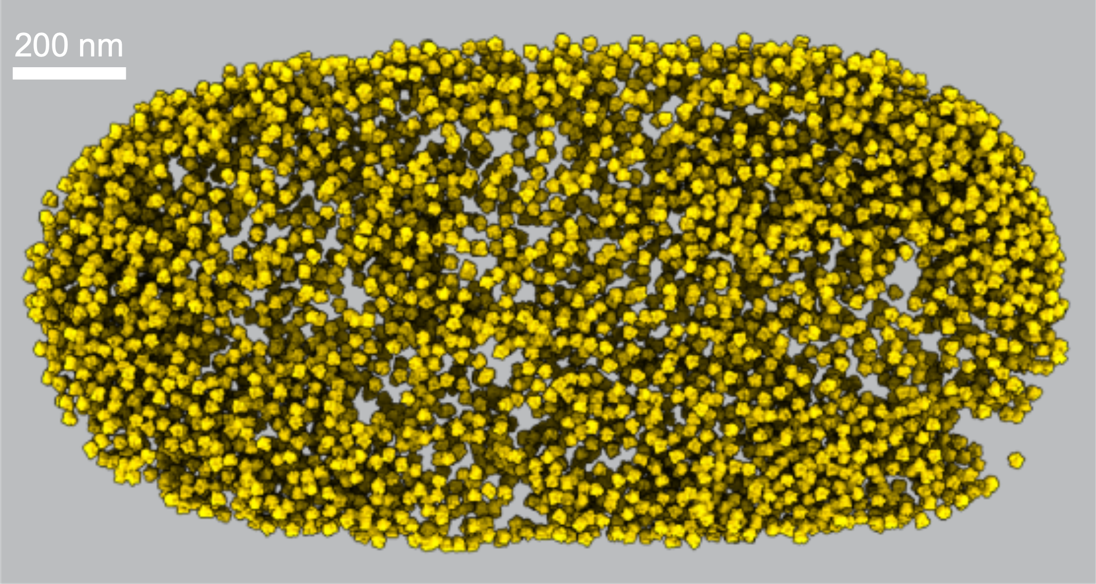 The density of E. coli ribosomes inside a cell, inferred from cryo
electron tomography data.
Source: Xiang et al (2020).
The density of E. coli ribosomes inside a cell, inferred from cryo
electron tomography data.
Source: Xiang et al (2020).
Making ribosomes fast enough for the cell to make a new daughter cell every 20 minutes (with 10K-50K new ribosomes) is a serious engineering challenge for E. coli. A ribosome is composed of two subunits, small and large. The large subunit contains LSU (large subunit) rRNA, 5S rRNA, and 33 ribosomal proteins; small subunit contains SSU (small subunit) rRNA and 21 ribosomal proteins. Ribosomal protein genes are highly expressed as mRNAs, but they also have the advantage that translation then makes about 50 proteins per mRNA. The ribosomal RNAs get no such amplification. The three rRNAs are about 2.9kb (LSU), 1.5kb (SSU), and 120nt (5S), totaling about 4.5kb of noncoding RNA that needs to be made to make one ribosome. This multiplies out to about 225Mb of rRNA needed to make 50K ribosomes, and that means making new rRNA at about 200Kb per second (assuming a 20' division time). One RNA polymerase transcribes at about 50nt/second. The size of the RNA polymerase (just a little smaller than a ribosome) occupies about 50nt on the gene it's transcribing. If we absolutely pack 4.5kb of an rRNA gene locus full with transcribing RNA polymerase, we can put a maximum of 4500/50 = 90 polymerases to work at 50nt/sec: we can get 4.5kb/sec of rRNA transcription. That's way short of 200Kb/sec. We have a problem - or rather, E. coli does.
E. coli solves this problem in two ways. One is brute force: amplify the number of genes. E. coli has seven rRNA operons, not just one: now we can get 4.5x7 \(\simeq\) 30kb/sec, which is still a factor of 7x short of engineering specs. Mammalian cells have hundreds of rDNA repeats for this same reason. Making rRNA fast enough is a big engineering concern in all cells.
The second way is weird and beautiful. E. coli starts rounds of DNA
replication asynchronously with cell division. It has to, because it
takes 60' for DNA polymerase to replicate the genome, but E. coli
divides every 20'. The genome
is a
circular chromosome with the origin of replication at the top (as we
draw it) and the replication termination region at the bottom.
It starts a new round of replication every 20' at the origin -
creating new replication forks moving bidirectionally down the
circle. At the origin, there are already about 3 rounds of replication
ongoing, which means there are about 2\(^3\) = eight copies of any locus
near the origin. (Whereas there's only about one copy of each locus
near the terminator.) So E. coli can place its genes accordingly,
to optimize gene copy number, and it smartly places its rRNA operons
near the origin to get the benefit of this replication-dependent
amplification.
This works out to about 4000 RNA polymerases hard at work making rRNA transcripts. Turns out that there are about 8000 RNA polymerases total in the cell, leaving 4000 for making protein-coding mRNAs.
There are about 8000 mRNAs in the cell. This immediately leads to another fun fact: the mean number of mRNAs per gene in one bacterial cell is only about one or two!
Each mRNA is about 1-2kb in size, so the total length of mRNA is around 8-16Mb, whereas the total length of ribosomal RNA in the cell is around 50k x 4.5k = 225Kb. This means that the RNA content of a cell is dominated by rRNA (and tRNA). Messenger RNA is only a minor fraction.
Moreover, ribosomal RNA is very stable (ribosomes are expensive to make), while in contrast, mRNA is unstable, with a halflife of only about 5 minutes. It makes sense for mRNA to have a stability less than a division cycle, so that transcriptional regulation is capable of altering mRNA levels (especially downward) quickly relative to the cell's life.
To maintain a steady state level of about 1-2 mRNA molecules per cell, with them decaying with a halflife of about 5 minutes, a new mRNA needs to be synthesized a typical gene about every 7 minutes. We'll firm up the necessary equations in the next section.
steady state expression levels
Let's suppose, as an approximation, that mRNA levels in a cell are at steady state. (That is, let's neglect dilution caused by cell growth and division.) Let's also assume that there are only two steps controlling mRNA levels: mRNAs are synthesized at rate \(k_1\) (in mRNAs/min/cell), and mRNAs decay at rate \(k_2\) (in min\(^{-1}\)). Steady state is when the number of new mRNAs synthesized equals the number that decay:
so at steady state,
So if the synthesis rate is 0.2 mRNAs/min/cell, and the mRNA decay rate is 0.2 min\(^{-1}\), then there is 1 mRNA/cell at steady state.
mRNA decay is more usually expressed by RNA biochemists in terms of the half life (in minutes, in bacteria; in hours, in mammalian cells), not as the decay rate. The half life is \(t_{1/2} = \frac{\ln 2}{k_2}\); and \(k_2 = \frac{\ln 2}{t_{1/2}}\).
If you block new transcription and measure only decay, then you get a classic exponential decay curve:
where \(f(t)\) is the fraction remaining at time \(t\).
You can derive this from a Poisson distribution. You can think of \(k_2 t\) is the expected number of "hits" that an mRNA molecule takes in time interval \(t\) minutes, at a rate \(k_2\) per minute; \(k_2 t\) is the expected number of hits in \(t\) minutes; and \(f(t)\) is the probability of zero hits after \(t\) minutes.
measuring mRNA expression level with RNA-seq
RNA-seq experiments are a paradigmatic example of large data sets in genomics. An RNA-seq experiment lets us measure the relative levels of all the RNAs in a sample of cells simultaneously -- or even in a sample prepared from a single cell, in what are called single-cell RNA-seq experiments (scRNA-seq).
Leaving aside a lot of molecular biology protocol voodoo, the essence of an RNA-seq experiment is to start with an RNA sample, make a library of DNA fragments corresponding to fragments of RNA in that sample, and sequence short (maybe 100-200nt) sequences from those fragments. We get a data set of 100-200nt sequence reads as a file. Computationally, we then map those reads back to the expected transcriptome (or the genome), in order to obtain a number of mapped read counts per transcript. From mapped read counts, we can infer relative mRNA abundance.
The result is often a tabular data file of samples by genes (or cells by genes, in scRNA-seq; or the transpose of these), where the values in the table are a measure of the observed abundance of each gene (mRNA) in the experiment. The measurements are either the mapped read counts, or in derived/inferred units of transcripts per million transcripts (TPM).
Let's work through this inference of TPM expression levels in terms of equations. Each gene \(i\) expresses some number of mRNA transcripts per cell. Let's call that actual number \(t_i\). I've already made a strong simplifying assumption -- that there's one mRNA per gene. In mammalian cells, I need to worry about alternative isoforms, including alternative splicing, alternative 5' initiation, and alternative 3' poly-A+ addition sites. In bacterial cells, I need to worry about operons, where one transcription unit encodes multiple protein-coding genes. In an RNA-seq experiment, we've usually taken our RNA sample from an unknown number of cells, so we're generally going to have to think in terms of relative proportions, not absolute numbers. In a large sample, the proportion of mRNA transcripts from gene \(i\) is \(\tau_i = \frac{t_i}{\sum_j t_j}\). These unknown \(\tau_i\) expression levels are what we aim to infer from observed counts of mapped reads.
In RNA-seq data processing, we map short sequence reads to annotated transcript sequences, which gives us a number of mapped reads per transcript: \(c_i\). The proportion of mapped reads that mapped to transcript \(i\) is \(\nu_i = \frac{c_i}{\sum_j c_j}\). People sometimes call the \(\nu_i\) the nucleotide abundance.
However, in typical RNA-seq experiments, we sequenced fragments (with short-read sequencing), not the whole mRNA or a specific end of it, so there's a bias from the mRNA length. Longer mRNAs give us more fragments, so they're overrepresented in the experiment. So to infer \(\tau_i\) from observed mapped read counts \(c_i\), we need to weight the counts inversely with the mRNA length \(\ell_i\):
The inferred \(\hat{\tau}_i\) is a fraction between 0 and 1 for each mRNA \(i\). To get this into units that are easier to think about, we then multiply by \(10^6\) and report transcripts per million transcripts (TPM).
In mammalian cells, which typically have around 100K-1M mRNA transcripts, TPM units are roughly equal to mRNA/cell. In bacterial cells, with a few thousand mRNAs/cell, TPMs don't have that nice intuition. A typical E. coli gene expressed at about 1-2 mRNA/cell will show up with a TPM of about 100-200 TPM.
Pandas
One of our goals this week is to introduce you to Pandas. Among other things, Pandas gives you powerful abilities to manipulate 2D tables of data, especially tidy data in the Wickham sense.
See also:
- online Pandas documentation
- The book Python for Data Analysis, by Wes McKinney, the author
of Pandas.
[website] [amazon]
The usual import aliases Pandas to pd:
import pandas as pd
creating a pandas DataFrame
A Pandas DataFrame is a 2D table with rows and columns. The rows and columns can have names, or they can just be numbered \(0..r-1\), \(0..c-1\).
You can create a DataFrame from a 2D array (a Python list of lists, or a numpy array), with default numbering of rows and columns, like so:
# create a data table with 4 rows, 3 columns:
D1   =  [[  2.0, 17.0, 15.0 ],
         [  3.0, 16.0, 12.0 ],
         [  4.0, 19.0, 11.0 ],
         [  5.0, 18.0, 10.0 ]]
df1  = pd.DataFrame(D1)
Or you can create one from a dict of lists, where the dict keys are the column names, and the list for each key is a column.
D2 = { 'lacZ': [ 12.0, 16.0,  4.0, 8.0 ],
       'lacY': [  7.0, 21.0, 14.0, 28.0],
       'lacA': [  5.0, 25.0, 20.0, 10.0] }
df2 = pd.DataFrame(D2)
Pandas calls the row names an index, and it calls the column names, the, uh, column names. You can set these column and row numbers with lists either when you create the DataFrame, or by assignment any time after. For example:
df1 = pd.DataFrame(D1,
                   index=['sample1', 'sample2', 'sample3', 'sample4'],
                   columns=['atpA','atpB','atpC'])

df2 = pd.DataFrame(D2,
                   index=['sample1', 'sample2', 'sample3', 'sample4'])

df1.index   = ['sample1', 'sample2', 'sample3', 'sample4']
df1.columns = ['atpA','atpB','atpC']
Try these out in a Jupyter notebook page - type df1 or df2 on its
own in a cell and Jupyter will show you the contents of the object
you've created.
reading tabular data from files
The pd.read_table() function parses data in a file:
df = pd.read_table('file.tbl')
By default, read_table() assumes tab-delimited fields. You will also
encounter comma-delimited and whitespace-delimited files commonly. You
specify an alternative single-character field separator with a
sep='<c>' argument, and you can specific whitespace-delimited with a
sep='\s+' pattern-matching argument.
   df = pd.read_table('file.tbl', sep=',')    # comma-delimited file. Same as pd.read_csv()
   df = pd.read_table('file.tbl', sep='\s+')  # whitespace-delimited file
Column names: by default, the first row is assumed to be a header containing the column names, but you can customize:
  df = pd.read_table('file.tbl')                         # First row is parsed as column names
  df = pd.read_table('file.tbl', header=None)            # There's no header. Don't set column names, just number them
  df = pd.read_table('file.tbl', header=5)               # The sixth row contains the column names (see: skiprows option)
  df = pd.read_table('file.tbl', names=['col1', 'col2']) # Assign your own list of column names
Row names: by default, Pandas assumes there are no row names (there are
\(n\) fields per line, for \(n\) column names), but if the first field
is a name for each row (i.e. there are \(n+1\) fields on each data line,
one name and \(n\) named columns), you use index_col=0 to assign which
column is the "index":
df = pd.read_table('file.tbl', index_col=0) # First field is the row name
To get Pandas to skip comments in the file, use the comment= option to
tell it what the comment character is:
df = pd.read_table('file.tbl', comment='#') # Skip everything after #'s
peeking at a DataFrame
    (nrows, ncols) = df.shape     # Returns 'shape' attribute of table: row x col dimensions
    df.dtypes                     # Summarize the data types used in each column
    df.info()                     # Show some summary info for a DataFrame
    df.head(5)                    # Returns first 5 rows
    df.sample(20)                 # Returns 20 randomly sampled rows
    df.sample(20, axis=1)         # Returns 20 randomly sampled columns
indexing rows, columns, cells in a DataFrame
The best way to learn is to play with example DataFrames in a Jupyter notebook page. I find Pandas to be inconsistent and confusing (sometimes you access a DataFrame as if it's column-major, and sometimes like it's row-major, depending on what you're doing) but it's pretty powerful once you get used to it.
To extract single columns, or a list of several columns, you can index into the DataFrame as if it's in column-major form:
   df['lacZ']                 # Gets 'lacZ' column, as a pandas Series
   df[['lacZ','lacY']]        # Gets two columns, as a smaller DataFrame
As a convenience, you can also use slicing operators to get a subset of rows; with this, you index into the DataFrame as if it's in row-major form, and the slice operator behaves as you'd expect from Python (i.e. as a half-open interval):
   df[2:4]     # gets rows 2..3; i.e. a half-open slice interval [2,4)
   df[2:3]     # gets just row 2

   df[2]       # DOESN'T WORK: it will try to get a *column* named '2'!!
To access data by row/column labels, use the .loc[] method.
.loc takes two arguments, for which rows and columns you want to
access, in that order (now we're row-major again). These arguments are
the row/column labels: either a single label, or a list. Note
that .loc takes arguments in square brackets, not parentheses! Also
note that when you use slicing syntax with .loc, it takes a closed
interval, in contrast to everywhere else in Python where you'd expect
a half-open interval.
   ## When rows are labeled:
   df.loc['sample1']                         # Extracts row as a Series (essentially a list)
   df.loc[['sample1','sample2']]             # Extracts two rows

   ## When rows are numbered, not labeled with an index, .loc will work:
   df.loc[2:3]                               # Extracts two rows when rows are numbered, not labeled. Note, closed interval!!
   df.loc[2:3, ['lacZ', 'lacY']]             # Extracts rows 2..3, and these two columns
   df.loc[2,'A2M']                           # Get a single value: row 2, column 'A2M'
To access data by row/column positions, use the .iloc[]
method. .iloc[] has square brackets around its row/col arguments
just like .loc[] but the arguments are an integer, a list of
integers, or a range like 2:5. Ranges in .iloc[] are half-open
intervals; compare:
Did I mention yet, Pandas is great and super-useful and all, but well-designed
and consistent? Well, you can't have everything. Just get used to it and keep good crib notes.
    df.loc[2:3]      # By label, closed interval: gets rows 2..3
    df.iloc[2:3]     # By index, half-open interval: gets row 2
getting, or iterating over row and column labels
   df.index              # Gets row labels, as an index object
   df.columns            # Gets column labels, as an index object
   list(df)              # Gets column labels as a list, sure why not
   [c for c in df]       # Example of iterating over column labels (as a list comprehension)
   [r for r in df.index] #   ...or of iterating over row labels
sorting data tables
The sort_values()
method gives you a wide range of sorting abilities.
The by= option tells it what field to sort on (which column label,
usually). The argument to by= is a single column label (a string),
or a list of them. If it's a list, it sorts first by the first one,
then second by the second, etc.
By default, it sorts rows, by some column's value. If you choose 'axis=1', it sorts columns, by some row's value.
By default, it sorts in ascending order; specify ascending=False to
get descending order.
df_sorted = df.sort_values(by='lacZ', ascending=False)
melting data tables
The method for melting a wide-form data table to a long-form one is
melt
For example, if I had a wide-form table of RNA-seq data with a column for the gene name, followed by a bunch of columns for different samples, I could keep the gene name column and melt the rest of the table to two new columns called "sample name" and "tpm":
df_long = pd.melt(df_wide, id_vars=['gene'], var_name='sample name', value_name='tpm')
If my gene names were the index of the DataFrame instead of a column,
I'd add the ignore_index=False argument to get pd.melt() to use
the same index in making the new melted DataFrame.
merging data tables
Suppose you have two data tables with different columns for the same rows (genes).
...like in the pset this week...
You can integrate the data tables into one using the
concat
or
merge
methods.
concat is mostly intended to concatenate additional rows onto a
table: i.e. merging tables that have the same columns, to create a
longer table. But it has an axis= argument (as in numpy) that lets
you concatenate horizontally. If the two tables share the same index
row names, this is as simple as:
df_concat = pd.concat([df1, df2], axis=1) # note it takes a list of DataFrames as its arg
merge is more powerful (I think) and intended not only for integrating
data frames horizontally (same rows, adding new columns), but also for
dealing with how exactly you want to handle various cases of the indexes (or column to use
as the key for the merge) not exactly matching. In good times, it is as simple as:
df_merge = pd.merge(df1, df2, on='gene_name')
where the on='gene name' tells the merge to use that column for the integration. If
I want to merge on a common index, I instead use:
df_merge = pd.merge(df1, df2, left_index=True, right_index=True)
plotting example
To scatter plot two columns against each other (i.e. each row is a point on the scatter plot):
ax = df.plot(kind='scatter', x='lacZ', y='lacA')
But you can also just pull out the columns you want to use as data (for plotting lines, or scatter plots, or a categorical column as the x-axis for a boxplot or Seaborn stripplot of a distribution on the y-axis), and pass them to matplotlib/Seaborn plotting functions as data. That's what I usually do (and that's all that Pandas is doing internally too).