week 04: sequence alignment

Cryptography has contributed a new weapon to the student of unknown scripts.... the basic principle is the analysis and indexing of coded texts, so that underlying patterns and regularities can be discovered. If a number of instances are collected, it may appear that a certain group of signs in the coded text has a particular function...
- John Chadwick, The Decipherment of Linear B

sequence similarity and homology

One of the most fundamental things we do in computational sequence analysis is to compare sequences using sequence alignment.

Sequences that are evolutionarily related by descent from a common ancestor are called homologous. We infer homology from sequence similarity. When two sequences are more similar to each other than we expect by chance, it's usually a good bet that they are homologous.

The alternative explanation for significant sequence similarity is some sort of convergent evolution, where the sequences have been driven to be similar by similar selective pressures. The space of possible sequences is so enormous that convergent evolution is typically only a concern for relatively simple and/or repetitive sequence motifs. Alpha-helical coiled-coil domains are one good example where people believe there's been multiple occurrences of convergent evolution to the same structure.

There are plenty of pitfalls in assuming that homologous sequences have related functions. Sequences can change their function dramatically in the course of evolution, just like related words can change their meaning in the evolution of languages. But just as in etymology of words, the exceptions sort of prove the rule; the history of where the sequence came from usually provides an illuminating clue. If we obtain a new DNA or protein sequence of unknown function from somewhere, an easy way to get a clue about its function (if any) is to search a sequence database for homologs in known sequences. If the new sequence is homologous to a sequence of known function that's already been studied, the new sequence probably has a related function.

Depending on how strongly a sequence is constrained by selective pressure, it may evolve slowly or quickly. Sequences that are under no selective pressure at all evolve at the neutral rate, which for mammalian genomes is very roughly about 1% substitution per position per million years. In comparisons of mammalian genomes separated by maybe up to 20 million years, we can align even neutrally evolving DNA sequence and infer things about the mutation rate and fixation rates in populations. As we compare more and more distantly related genomes, sequences have to be more strongly conserved to be detected by similarity searches. Some of the most highly constrained protein sequences, such as histones, have only accumulated a small handful of amino acid substitutions over many hundreds of millions of years.

One of the great surprises of molecular biology and genomics was that protein and DNA sequences are startlingly similar, across great gulfs of evolutionary time. We can readily identify homologous genes across humans, flies, worms, yeast, and bacteria. Computational sequence comparisons have immense power.

Sequences evolve in other kinds of steps too, but standard primary sequence alignment neglects them. Foe example, a single mutation event can change multiple residues at once. This happens commonly with some DNA repair and recombination mechanisms, such as gene conversions. Nonlinear rearrangements like duplication, transposition, and inversion happen too, and become very non-neglectable at larger (chromosome/genome) length scales. If we assume that sequences evolve in steps of single-residue ("point") substitutions, insertion of one or more residues, or deletions of one or more residues, then the detailed evolutionary relationship between two or more sequences can be compactly represented in a linear alignment, with homologous residues aligned in columns.

These alignments are taken from a figure in the book Biological Sequence Analysis by Durbin, Eddy, Krogh, and Mitchison (1998). The figure below shows an example of three pairwise sequence alignments to a piece of human $\alpha$-globin, HBA_GLOBIN.

HBA_HUMAN  GSAQVKGHGKKVADALTNAVAHVDDMPNALSALSDLHAHKL
           G+ +VK+HGKKV  A+++++AH+D++ +++++LS+LH  KL
HBB_HUMAN  GNPKVKAHGKKVLGAFSDGLAHLDNLKGTFATLSELHCDKL

HBA_HUMAN  GSAQVKGHGKKVADALTNAVAHV---D--DMPNALSALSDLHAHKL
           ++ ++++H+ KV   + +A  ++          +L+ L+++H+ K 
LGB2_LUPLU NNPELQAHAGKVFKLVYEAAIQLQVTGVVVTDATLKNLGSVHVSKG

HBA_HUMAN  GSAQVKGHGKKVADALTNAVAHVDDMPNALSALSD----LHAHKL
           GS+ + G +   +D L  ++ H+ D+  A +AL D    ++AH+ 
F11G11.2   GSGYLVGDSLTFVDLL--VAQHTADLLAANAALLDEFPQFKAHQE

The first alignment shows an unambiguous similarity to human $\beta$-globin. $\alpha-$ and $\beta-$ globin diverged maybe 600 million years ago when hemoglobin evolved by a gene duplication in the early vertebrate evolution. The '+' symbols in the alignment mark columns where the amino acid substitution is considered to be conservative. (The score matrix used in the comparison gave this pair a nonnegative score.)

The last alignment shows a "similarity" that occurs by chance to a nonhomologous protein sequence, a C. elegans glutathione S-transferase. It's typical to find similarities by chance that look like this, at about 20% identity or so (for protein alignments).

The alignment in the middle doesn't look much different from the last one, but it's to a real globin homolog: LGB2_LUPLU is a plant leghaemoglobin (from yellow lupin). Both plants and animals use globins for oxygen binding. Plants and animals diverged about 1-2 billion years ago. This is an example of a remote homolog, difficult to detect by pairwise sequence similarity alone.

finding and scoring alignments

Let's concentrate on pairwise sequence alignment for now. More sophisticated things like profile alignment and multiple sequence alignment are conceptually similar, and we can see the basics first.

We need two things: a mathematical way to score alignments and distinguish alignments of true homologs from chance, and once we have a good scoring function, we need an algorithm for identifying high-scoring alignment(s).

In the early days of sequence alignment, people assigned +1 to an identity, -1 to a mismatch, and some "gap penalty" for introducing an insertion or deletion.

We can do much better than simple sequence identity by incorporating more information about residue conservation. In proteins, for example, we want to capture information about structural and chemical similarity between amino acids -- for example, a K/R mismatch should be penalized fairly little (and maybe even rewarded) because lysine (K) and arginine (R) are both positively charged amino acids with similar roles in protein structures, whereas an R/V mismatch should probably be penalized fairly strongly because arginine and valine (V) are dissimilar amino acids that don't substitute for each other well. So, more generally, we can assign a score $\sigma(a,b)$ to a residue pair $a,b$ - $\sigma(a,b)$ can be high if $a$ and $b$ are an acceptable substitution, and low if not. We'll call $\sigma$ a substitution matrix or a score matrix.

We also need to worry about how best to score gaps. If we don't penalize our use of gaps somehow, our "optimal" alignments can get pretty unrealistic. The computer will insert lots of gap symbols trying to maximize the apparent similarity of the residues. In a pairwise sequence alignment, we can't tell the difference between an insertion in one sequence versus a deletion in the other; therefore we sometimes refer to gaps as indels, short for insertion/deletion. A fairly general kind of gap score is to assess a (negative) gap score $\gamma(n)$ every time we invoke a gap of length $n$ in an alignment, and have a big table for $\gamma(n)$ as a function of $n$. Generalized gap score functions are rarely used, because they lead to more computationally complex alignment algorithms. Instead, we typically use one of two simple functional forms that are more compatible with efficient recursive solutions. Linear gap penalties have the form $\gamma(n) = n \gamma$ - a linear cost of $\gamma$ units per gap character. Affine gap penalties have the form $\gamma(n) = \alpha + n \beta$ - $\alpha$ is a gap-open cost for the first residue, and $\beta$ is a gap-extend cost for each additional residue in the indel.

On the algorithm side now. Brute force enumerating all possible pairwise sequence alignments and ranking them is infeasible. There are about $\frac{2^{2L}}{\sqrt{2 \pi L}}$ possible global alignments between two sequences of length L. Some sort of efficient alignment algorithm is needed.

Dynamic programming algorithms for sequence alignment were borrowed from digital signal processing, where they're sometimes called dynamic time warping algorithms. Global alignment algorithms - aligning two sequences over their full length - were introduced to computational biology by Needleman and Wunsch in 1970, and are typically called Needleman/Wunsch algorithms even though the original algorithm used a generalized gap scoring function. Local alignment algorithms - finding the best-scoring match between any subsequences of two sequences - were introduced by Smith and Waterman in 1981, by a small but crucial modification to the Needleman/Wunsch algorithm. Local alignment algorithms are called Smith/Waterman algorithms. A series of fast heuristically accelerated versions of Smith/Waterman were introduced in the 1980's, leading to the widely used FASTA and BLAST software packages.

In what follows, I will introduce a series of algorithms that leads up to Smith/Waterman local alignment (and beyond), where we assume that the scoring system is given (substitution matrix $\sigma(a,b)$ and gap penalties). Then I'll come back to the scoring system, tell you where $\sigma(a,b)$ come from, and tease you with a bit about where the gap penalties ought to come from.

the lowly dotplot

For recognizing similarities between two sequences, one of the most basic visualizations is the dotplot. It also happens to be a good place to start understanding sequence alignment algorithms.

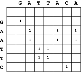
A dotplot of X=GAATTC against Y=GATTACA. In a dotplot, we draw a matrix with one sequence $X$ as the vertical axis and the other sequence $Y$ as the horizontal axis. (Either way works, but choose one and be consistent.) Each cell of this dotplot matrix $D(i,j)$ represents the alignment of one residue $X_i$ to one residue $Y_j$. For every identical pair of residues $X_i$ and $Y_j$, we put a dot (or some kind of mark - I'll put a 1) in the corresponding cell $D(i,j)$. Significant local alignments appear as strong diagonal lines in the resulting plot, against a random background of uncorrelated dots. An small and somewhat uninteresting example is shown in the figure to the right.

We can use the dotplot procedure to better introduce the Python-esque pseudocode notation I'll be using. Given two sequences $X$ and $Y$, the algorithm to construct the dotplot matrix $D$ is as follows:

def dotplot(X,Y):
    L = len(X)
    M = len(Y)

    for i = 1 to L:
        for j = 1 to M:
            if X(i) == Y(j):  D(i,j) = 1
            else:             D(i,j) = 0
    return D

Dotplot of PABP_DROME against itself, revealing that it has an internally duplicated structure.

The lowly dotplot introduces some ideas: the 2D matrix representation of comparing and aligning a pair of sequences; that an alignment corresponds to a diagonal in the matrix; and what my algorithm pseudocode is going to look like.

But even the lowly dotplot, barely worth calling an "algorithm", is useful as a visualization in sequence analysis. For example, the figure to the right shows a dotplot comparison of Drosophila poly-A binding protein to itself, showing three strong off-diagonal striations that are a dead giveaway that this protein has four repeated domains: four RNA recognition motif domains (RRMs), as it happens. Larger scale DNA dotplots easily visualize inversions, transpositions, and duplications that primary sequence alignment algorithms can't easily deal with. (I produced this dotplot with dotter, a package from Erik Sonnhammer, which uses a dotting rule that's a little more sophisticated than what I just described; dotter looks along and scores local diagonals before assigning a score to a matrix cell.)

longest common substring

With a small modification to the dotplot algorithm, we convert it into an algorithm that finds the longest common substring (LCS) that the two strings $X$ and $Y$ have in common (i.e. completely identical). For example, the LCS of GATTACA and GAATTC is ATT, 3 letters long. The LCS algorithm is as follows:

def LCS(X,Y):
    L = len(X)
    M = len(Y)

    # Initialization:
    D(0,0) = 0                   # upper left cell
    for i = 1 to L: D(i,0) = 0   # left column
    for j = 1 to M: D(0,j) = 0   # top row

    # Recursion:
    for i = 1 to L:
        for j = 1 to M:
            if X[i] == Y[j]:  D(i,j) = D(i-1,j-1) + 1
            else:             D(i,j) = 0

    # Termination:
    best_sc   = max_{ij} D(i,j)
    end_pos   = argmax_{ij} D(i,j)
    start_pos = end_pos - D(i,j) + 1

LCS alignment of X=GAATTC to Y=GATTACA.

An example matrix calculated by this algorithm is shown in the figure to the right.

sidebar on "dynamic programming"

The word "programming" refers to the tabular matrix, not to computer code. another place this usage might confuse you is the term "linear programming", a tabular method for solving systems of equations. The word "dynamic" means nothing. Dynamic programming was introduced by Richard Bellman in the 1950's when he was working on military contracts at RAND. The Secretary of Defense at the time was hostile to mathematical research. Bellman explained in his autobiography, "['Dynamic'] has a very interesting property as an adjective, and that is it's impossible to use the word dynamic in a pejorative sense. Try thinking of some combination that will possibly give it a pejorative meaning. It's impossible. Thus, I thought dynamic programming was a good name. It was something not even a Congressman could object to.".

The LCS algorithm is a simple example of what are called dynamic programming algorithms. Scoring $D(i,j)$ required that we know $D(i-1,j-1)$. Our solution is recursive. We solve smaller problems first, and use those solutions to solve larger problems. We know what problems are smaller (and already calculated) by our position in the tabular matrix $D$. Computer scientists refer to a recursive method that stores the results of intermediate solutions in a tabular matrix as a dynamic programming method.

Dynamic programming methods have to worry about boundary conditions. You can't start recursing until you've defined the smallest solutions non-recursively. A DP algorithm typically has an initialization phase for this. In sequence alignment, it typically means initializing a top row 0 and left column 0 of the alignment matrix.

In dynamic programming sequence alignment, after a stage where we fill the matrix (typically from upper left to bottom right), there's a termination phase where we find the optimal score: perhaps in the bottom right corner (for global alignment), in the rightmost column (for alignments that are global in sequence $Y$ but local in $X$), or anywhere in the matrix (for local alignments, including the LCS algorithm).

Having identified where the optimal score is, we also know the optimal alignment ends at that position, but we don't yet know where it started. For that, dynamic programming algorithms have a traceback phase where we reconstruct the optimal path backwards step by step through the matrix. In the case of the LCS algorithm, the traceback is trivial because the score $D(i,j)$ itself tells us how long the optimal diagonal is: if the optimal $D(i,j)$ is 3, then my optimal start was at $(i-2,j-2)$. In the gapped sequence alignment algorithms we'll soon see, it's less trivial.

sidebar on big-O notation

We're often concerned with comparing the efficiency of algorithms. A natural way to measure the efficiency of an algorithm is to show how required computational resources (both running time and memory) will scale as the size of the problem increases. Problem sizes can often be measured in number of units, $n$. For instance, in sequence alignment, we will measure problem sizes as the length of one or more sequences in residues.

Generally computer scientists will state the efficiency of an algorithm by analyzing its asymptotic worst-case running time. If an algorithm is guaranteed to take time proportional to the square of the number of units in the problem (or less), for instance, we say that the algorithm is $O(n^2)$ (slangily, "order n-squared") in time. This $O()$ notation is called "big-O" notation.

Sharpening that up: The real running time of an algorithm (in units of steps) is a function $f(n)$ of the problem size $n$. We expect $f(n)$ to increase monotonically with increasing $n$, though not necessarily in a simple way. Some problems of the same size might be easier to solve than others, and ouralgorithm might have different stages with different complexity (like, a startup cost associated with initializing some stuff, followed by the main computation). But asymptotically as the problem size $n$ increases toward infinity, and for the worst case problem, we can define a simple function $g(n)$ such that there are constants $c$ and $n_0$ such that $c g(n) >= f(n)$ for all problems of size $n > n_0$. We then say that the algorithm is $O(g(n))$.

An $O(n^k)$ algorithm is called a polynomial time algorithm. So long as $k$ is reasonable (3 or less) we will usually speak of the problem that this algorithm solves as tractable. Pairwise sequence alignment algorithms - even the dotplot! - are typically $O(n^2)$.

An $O(k^n)$ algorithm (for some integer k) is called an exponential time algorithm, and we will be reluctant (if not horrified) to use it. Sometimes we go so far as to call the problem intractable if this is the best algorithm we have to solve it. However, we can often find heuristic shortcuts and settle for reasonable solutions, albeit less-than-optimal ones, for problems that require exponential time to solve optimally.

Some problems have no known polynomial time solutions. An important class of problems are so-called NP (nondeterministic polynomial) problems.

In general, we will tend to believe that an $O(2^n)$ algorithm is inferior to an $O(n^3)$ algorithm, which is inferior to an $O(n^2)$ algorithm, which is inferior to an $O(n \log n)$ algorithm, which is inferior to an $O(n)$ algorithm. However, $O()$ notation, though ubiquitous and useful, must be used with caution. A superior $O()$ does not necessarily imply a faster running time, and equal $O()$'s do not imply the same running time.

Why not? Well, first there's that constant $c$. Two $O(n)$ algorithms may have quite different constants, and therefore run in quite different times. Second, there's the notion (embodied in the constant $n_0$) that $O()$ notation indicates an asymptotic bound, as the problem size increases. An $O(n)$ algorithm may require so much precalculation and overhead relative to an $O(n^2)$ algorithm that its asymptotic speed advantage is only apparent on unrealistically large problem sizes. Third, there's the notion that $O()$ notation is a bound for the worst case. We will see examples of algorithms that have poor $O()$ because of a rare worst case scenario, but their average-case behavior on typical problems is much better. Fourth, it's not the case that each computation step takes the same real time. Especially on modern computers, memory access time is typically rate-limiting, and an algorithm or implementation that accesses memory in a more architecture-friendly way (namely, in stride, where memory accesses are adjacent) can be much faster than one that has to access memory randomly.

Memory complexity is discussed in the same way. Pairwise sequence alignment algorithms are typically $O(n^2)$ in time, $O(n^2)$ in memory as they're presented in textbooks. In actual implementations, there are commonly-used tricks to get down to $O(n)$ memory.

We can define problem sizes with more than one variable. For example, with pairwise sequence comparison of two sequences of quite different lengths $L$ and $M$, we might specifically say that sequence alignment algorithms are $O(LM)$ in time and memory.

There can be additional subtleties to $O()$ notation, related asymptotic notations, and algorithmic analysis in computer science. For example, we casually assumed that our computing machine performs its basic operations (addition, subtraction, etc.) in $O(1)$ time, but strictly speaking this isn't true. The number of bits required to store a number $n$ scales with $\log n$, so for extremely large $n$, when numbers exceed the native range of 32-bit or 64-bit arithmetic on our computing machine, it will no longer take $O(1)$ time to perform storage, retrieval, and arithmetic operations. Such concerns are beyond the realm of computational biology and more in the realm of careful computer science theory.

The LCS algorithm is $O(n^2)$ for two strings of lengths $\sim n$. Much more efficient $O(n)$ LCS algorithms are possible, using suffix trees for example. The reason to show the less efficient LCS algorithm is purely pedagogical, a stepping stone on our way to dynamic programming sequence alignment algorithms that allow insertions and deletions.

global alignment: Needleman/Wunsch/Sellers

Now let's look at global sequence alignment. What is the best pairwise alignment between two complete sequences (including gaps), and what is its score?

The original 1970 Needleman/Wunsch global sequence alignment algorithm is an $O(n^3)$ algorithm that uses an arbitrary gap cost table $\gamma(n)$ for an indel of length $n$, but everyone forgets that. The version of the algorithm that's usually introduced in textbooks is a modification made by Peter Sellers (no, not that Peter Sellers) for a linear gap cost of $n \cdot \gamma$ that allows the algorithm to run in $O(n^2)$, and is also a simpler algorithm to understand.

We have our two sequences $X$ and $Y$, and we also are given a substitution scoring system $\sigma(a,b)$ (for the score of aligning a pair of residues $a,b$: 20x20 for protein, 4x4 for DNA), and a gap score per residue $\gamma$ (where $\gamma$ is negative, because it's a penalty).

The idea of the algorithm is to find the optimal alignment of the sequence prefix $X_1..X_i$ to the sequence prefix $Y_1..Y_j$. Let us call the score of this optimal alignment $F(i,j)$. ($F$ here stands for ``forward'' -- at some point you'll see why.) The key observation is this: I can calculate $F(i,j)$ easily if I already know $F$ for smaller alignment problems. The optimal alignment of $X_1..X_i$ to $Y_1..Y_j$ can only end in one of three ways:

• $X_i$ is aligned to $Y_j$.
  Now $F(i,j)$ will be the score for aligning those two residues, $\sigma(X_i,Y_j)$), plus the optimal alignment score I'd already calculated for the rest of the alignment prefixes not including them, $F(i-1,j-1)$.

• $X_i$ is aligned to a gap character.
  This means we're adding a gapped residue (which costs us a $\gamma$) to the optimal alignment we've already calculated for $X_1..X_{i-1}$ to $Y_1..Y_j$: so the score of this alternative is $F(i-1,j) + \gamma$.

• Or conversely, $Y_j$ is aligned to a gap character.
  The score of this alternative is $F(i,j-1) + \gamma$.

The optimal $F(i,j)$ is the maximum of these three alternatives.

Thus:

def nws(X, Y, sigma, gamma):
    L = len(X)
    M = len(Y)

    # Initialization:
    F(0,0) = 0                           # upper left cell
    for i = 1 to L: F(i,0) = gamma * i   # left column
    for j = 1 to M: F(0,j) = gamma * j   # top row

    # Recursion:
    for i = 1 to L:
        for j = 1 to M:
            F(i,j) = max { F(i-1,j-1) + sigma(X_i,Y_j),
                           F(i-1,j)   + gamma,
                           F(i,j-1)   + gamma  }

    # Termination:
    return F(L,M)

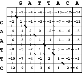
The dynamic programming matrix calculated for two strings GATTACA and GAATTC, using a scoring system of +1 for a match, -1 for a mismatch, and -2 per gap. The algorithm is $O(LM)$ in time and memory. When we're done, $F(L,M)$ contains the optimal alignment score. The figure to the right shows a small example.

However, we don't yet have the optimal alignment. To get that, we perform a traceback in $F$ to find the path that led us to $F(L,M)$.

One way to trace back is by recapitulating the score calculations. We start in cell $(i=L,j=M)$ and find which cell(s) we could have come from, by recalculating the three scores for coming from $(i-1,j-1)$, $(i-1,j)$, or $(i-1,j)$ and seeing which alternative(s) give us the optimal $F(i,j)$. If the optimal path came from $(i-1,j-1)$ we align $X_i$ to $Y_j$; if the optimal path came from $(i-1,j)$ we align $X_i$ to a gap; and if the optimal path came from $(i,j-1)$, we align $Y_j$ to a gap. We move to that cell, and iterate this process until we've recovered the whole alignment.

Another way to trace back is to store a second matrix of "traceback pointers" when we do the DP fill, storing which of the three paths we used to get $F(i,j)$. Then to do the traceback we just follow those pointers backwards.

The traceback is linear time. The DP fill stage dominates the computational complexity of the procedure, as well as capturing the most important ideas for how the algorithm works.

local alignment: Smith/Waterman

A local alignment is the best (highest scoring) alignment of any substring of $X$ to any substring of $Y$, as opposed to a global alignment of the entire strings. Local alignment is usually more biologically useful. It is usually the case that only part of two sequences is significantly similar, so those parts must be identified.

The Smith/Waterman algorithm adds a small but crucial step in the algorithm, allowing the local alignment to restart at any cell by adding a zero to the recursion, just as we already saw in the LCS algorithm. Temple Smith jokes that the most important result of his career was a zero.

def sw(X, Y, sigma, gamma):
    L = len(X)
    M = len(Y)

    # Initialization:
    D(0,0) = 0                   # upper left cell
    for i = 1 to L: D(i,0) = 0   # left column
    for j = 1 to M: D(0,j) = 0   # top row

    # Recursion:
    for i = 1 to L:
        for j = 1 to M:
            F(i,j) = max { 0,
                           F(i-1,j-1) + sigma(X_i,Y_j),
                           F(i-1,j)   + gamma,
                           F(i,j-1)   + gamma  }

    # Termination:
    return max_{ij} F(i,j)

After filling the $F$ matrix, we find the optimal alignment score and the optimal end points by finding the highest scoring cell, $\max_{i,j} F(i,j)$. To recover the optimal alignment, we trace back from there, terminating the traceback when we reach a cell with score $0$.

For Smith/Waterman to give local alignments, the scoring system $\sigma(a,b)$ must obey two conditions. At least one of the scores must be positive (favorable), and the overall expected score by chance, $\sum_{ab} f_a f_b \sigma(a,b)$, must be negative (unfavorable) - where $f_a$ and $f_b$ are the frequencies that residues $a$ and $b$ occur in sequences. These conditions are fulfilled automatically when score matrices are calculated as log-likelihood ratios, as described at the end of these notes.

affine gap penalties: Gotoh

Linear gap costs aren't very good. The field has generally settled on using an "affine" gap cost where it costs us a larger "gap-open" score $\alpha$ for opening the gap with its first residue, and a smaller "gap-extend" penalty $\beta$ for each successive residue.

The dynamic programming algorithm now needs to keep track of three states per cell: the optimal alignment given that we ended in a "match" (an alignment, match or mismatch), "insert", or "delete". We'll call these three states M, I, and D.

def sw_affine(X, Y, sigma, alpha, beta):
    L = len(X)
    M = len(Y)

    # Initialization:
    for i = 0 to L:       # left column
        M(i,0) = 0   
        I(i,0) = -infty
        D(i,0) = -infty
    for j = 1 to M: 
        M(0,j) = 0
        I(0,j) = -infty
        D(0,j) = -infty

    # Recursion:
    for i = 1 to L:
        for j = 1 to M:
            M(i,j) = sigma(X_i,Y_j) + max { 0,
                                            M(i-1,j-1),
                                            I(i-1,j-1),
                                            D(i-1,j-1) }

            I(i,j) = max { M(i-1,j) + alpha,
                           I(i-1,j) + beta  }

            D(i,j) = max { M(i,j-1) + alpha,
                           I(i,j-1) + beta }

    # Termination:
    return max_{ij} M(i,j)

more complex algorithms: the rise of the machines

You might find it hard to see what the affine-gap Smith/Waterman/Gotoh algorithm is doing. If you stare at it for a while, you can convince yourself that it's doing the right thing. For example, you can keep extending an existing insertion by being in the insert state already (where being in that state means you've already paid the gap-open cost), and extending by an additional $\beta$ cost. But there's an easier way: to see the problem graphically, as a finite state machine.

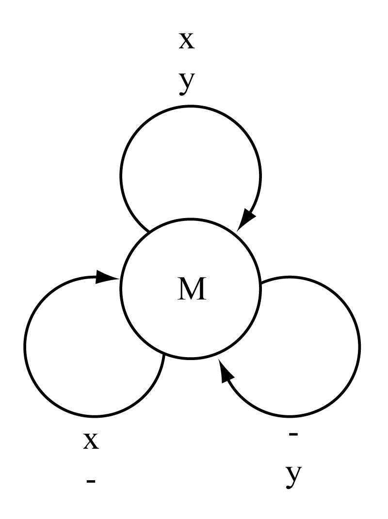
The Needleman/Wunsch/Sellers algorithm represented as a finite state machine. The figure to the right shows the machine representation of the NWS global alignment algorithm.

A machine is composed of one or more states, connected by state transitions. Here we have only one state, and three possible transitions representing an alignment, an insertion, and a deletion. We can either think of the machine generating alignments, or consuming them, one aligned column at a time.

Machine steps can either generate on transition or on state. This machine generates on transitions. An example of generating on state follows below. There's no reason one can't use both modes in a one machine.

When the machine uses the align transition (top), it generates a residue in sequence $X$ aligned to a residue in sequence $Y$, and pays a cost of $\sigma(a,b)$ for those two residues. When it uses the insert transition (left), it generates a residue in sequence $X$ aligned to a gap, and pays a cost of $\gamma$. When it uses the delete transition (right), it generates a gap aligned to a residue in sequence $Y$, and pays a cost of $\gamma$.

Converting a machine into a dynamic programming recursion goes as follows. We need one matrix for every machine state: here, one $M(i,j)$ matrix. We are going to compute "what is the probability that we are in state M after having generated the prefixes $X_1..X_i$ and the prefix $X_1..Y_j$?" To calculate that number $M(i,j)$, we maximize over each transition that could get us back into state $M$. Here, three possibilities. The score for using a transition is constructed by adding up the cost of any residues emitted by the state, plus the cost of any residues emitted by the transition, plus any cost associated with using the transition, plus (the key!) the score of whatever state the transition came from, at the appropriate $i,j$ coordinate that takes into account how many residues this transition generated in sequences $X$ and $Y$. For example, the align transition generates one residue in $X$ and one residue in $Y$, so it is assessed its score $\sigma(a,b)$ for those two residues and it "connects to" matrix cell $M(i-1,j-1)$. The insert transition generates one residue in $X$ and none in $Y$, so it is assessed its insertion score $\gamma$ (the residue itself is emitted for free in this model), and it connects to matrix cell $M(i-1,j)$. Thus, we construct the dynamic programming recursion:

M(i,j) = max { 0,
               M(i-1,j-1) + sigma(X_i,Y_j),
               M(i-1,j)   + gamma,
               M(i,j-1)   + gamma  }

The power of the machine representation is that you can draw what you want your alignment model to capture, then convert it to a DP recursion. I find it easier to draw a complex model than to prove a complex DP recursion.

affine gap alignment as a machine

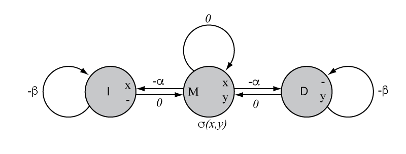The affine-gap Needleman-Wunsch global alignment algorithm represented as a finite state machine.

The figure at the right shows the machine representation of the more affine-gap global alignment algorithm. I've drawn this machine to emit on state, instead of emitting on transition. (You could draw an equivalent model that emitted on transition, if you wanted to.)

Visualizing the affine-gap-scoring problem as "entering the insertion state" in a machine make it more clear why the affine-gap versions of alignment algorithms require three matrices whereas linear-gap-penalty versions of these algorithm only needs one.

spliced alignment machine

What if we wanted to align two sequences under an even more complicated scoring scheme? For example, suppose we wanted to align a cDNA protein-coding sequence from one organism to a homologous genomic DNA sequence in another organism.

Quick review of the biology here: the genomic sequence of a eukaryotic gene is composed of segments called exons and introns. The gene is transcribed to produce a pre-mRNA transcript, which is spliced in the nucleus to remove all the introns, resulting in a mature mRNA (messenger RNA) that is exported to the cytoplasm, where ribosomes will translate it to produce protein. A cDNA (complementary DNA) is an artificial copy of a mature mRNA sequence, isolated and cloned in the lab. cDNA sequence libraries are a common way of sampling the sequences of mRNAs present in a cell.

One important feature of the cDNA/genomic alignment problem is that we expect the genomic sequence to require long insertions, because of the introns that the cDNA doesn't have. This adds a different reason for gaps in the alignment, in addition to insertions and deletions (indels) that occurred during sequence evolution. We expect introns to have different statistical properties than indels, so it's natural to want to model introns by a different gap penalty system. Moreover, we want that gap penalty to be applied asymmetrically, allowing introns only in the genomic sequence, not in the cDNA sequence.

A second feature of coding cDNA/genomic alignment (or rather, any alignment of protein-coding DNA sequences) is that coding regions are composed of codons, base triplets encoding amino acids, and the statistical properties of coding alignments are strongly affected by coding constraints. It is desirable to score a codon aligned to a codon, rather than treating this as three independent pairwise residue alignments. Insertions and deletions in a coding sequence almost always occur in lengths that are a multiple of three, to preserve the reading frame, and intron location must also preserve the triplet reading frame.

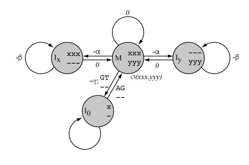
How would you extend the Needleman/Wunsch/Sellers dynamic programming algorithm to align the coding portion of a cDNA to a genomic sequence of two homologous genes, if I gave you: a) a scoring matrix $\sigma(xxx,yyy)$ for aligning two homologous triplet codons; b) a gap-open and gap-extend penalty $\alpha, \beta$ for scoring indels in either sequence in units of triplets; and c) an additional cost $\gamma$ for inserting an intron of any length, while enforcing a restriction that introns must start with a consensus GT and end with a consensus AG?

If you can see the correct answer immediately in terms of dynamic programming recursions, you are a demigod. For mortals, it is useful to draw it first as the state machine on the right.

The machine then guides us in how to construct the recursion (leaving out the initialization for clarity here):

M(i,j) = sigma(X(i-2,i-1,i), Y(j-2,j-1,j) + max { M(i-3,j-3),
                                                  IX(i-3,j-3)
                                                  IY(i-3,j-3),
                                                  I0(i-5,j-3) if X(i-5,i-4) == "AG" else -infty}

IX(i,j) = max { M(i-3,j) + alpha,
                IX(i-3,j) + beta }

IY(i,j) = max { M(i,j-3) + alpha, 
                IY(i,j-3) + beta }

I0(i,j) = max { M(i-3,j) + gamma if X(i-3,i-2) == "GT" else -infty,
                I0(i-1,j) }

This model illustrates the main idea, but it's too simple for the actual biological problem. It only captures "phase 0" introns that occur exactly between two adjacent codons. We would need to add additional states for phase 1 and phase 2 introns that split a codon. It would then turn out to be difficult to score the split codon correctly, because the finite state machine moves left to right and "forgets" what it saw at the start of the codon, when it reaches the end of it after the intron.

It's a small step from finite state machines to probabilistic models. The scores in the state machine are arbitrary, and we're allowing some of them to be free. In a probabilistic state machine, all the transition options from a state have probabilities that have to sum to one, and all the possible emissions from a state have probabilities that have to sum to one. In the pset, this is why Holmes looks at a gap probability of 1/32 and immediately says that the additive gap cost should be $\log_2 \frac{1}{32}$ = -5 bits: he's an aficionado and he's seeing the probability model for generating a sequence alignment as the same thing as the model used to infer an alignment. (Taking the logarithm is just to get an additive scoring system, instead of multiplying probabilities.)

We'll see more about that step when we get some more probability theory (next week) and hidden Markov models (week 8). But for now, as a preview, let's see where substitution score matrices come from....

where substitution score matrices come from

There is a simple equation for calculating substitution matrix scores:

$$ \sigma(a,b) = \frac{1}{\lambda} \log_2 \frac{p_{ab}}{f_a f_b} $$

The number $p_{ab}$ is the probability that we see an alignment of residue $a$ and residue $b$ in true pairwise alignments.

$f_a$ and $f_b$ are the observed independent frequencies of residues $a$ and $b$. That is, how often we expect to find these residues just by chance.

The $\lambda$ constant is effectively just choosing the base of the logarithm. We can just set it $\lambda=1$, and our scores are in units of bits.

The derivation for why this is a good score to use comes from assuming a probability machine for an ungapped sequence alignment where each aligned pair is assumed to be independently generated with joint probability $p(a,b)$, and a null hypothesis where the two sequences are independent and each i.i.d. random with residue probabilities $f(a)$. The log-likelihood ratio score for this two-hypothesis comparison can be factored into independent terms for each alignment column $i$:

$$ \sum_i \log_2 \frac{p(X_i,Y_i)} {f(X_i) f(Y_j)} $$

where we see that those terms are the $\sigma(a,b)$ terms I asserted were the right way to make a substitution matrix.