homework 09: a mixture of five
One of the undergraduate researchers in the Holmes group, Wiggins, left the lab suddenly, protesting his stipend of one shilling a day. He left you a mess of his work in progress. He isn't responding to your emails, so you're doing some detective work of your own.
Some of Wiggins' last work was a set of single-cell RNA-seq experiments on phage-infected bacterial cells. You've found records from an experiment in which he was looking at expression levels of two genes, a host defense gene called defA and a phage anti-defense gene called kilA. Previous work had shown that defA and kilA are often both expressed at intermediate levels, but sometimes one or both genes can be expressed at high or low levels, defining five "infected cell types", resulting in different outcomes of the battle between molecular weaponry of the phage and host.
Wiggins' single cell RNA-seq dataset
You've found a data file where Wiggins had collected mapped read counts for defA and kilA in 1000 single infected bacterial cells. Because he expected five "cell types" in the data, he used K-means clustering, with K=5, to try to assign each cell to one of the five cell types. Then he would estimate the mean expression level (in mapped counts) of the two genes in each cell type, and the relative proportions of the cell types in the population.
However, it's obvious from a figure you found taped into Wiggins' notebook, not to mention the various profanities written on it, that the K-means clustering did not go as hoped. His visualization of his data does show five clear clusters, but his K-means clustering failed to identify them:
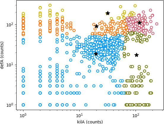 Figure 1: Wiggins' figure from his notebook, visualizing his K-means
clustering of the 1000 cells in his single cell RNA-seq
experiment, for K=5. Black stars indicate the five fitted centroids
from his best K-means clustering, and colors indicate the assignments
of the 1000 cells to the 5 clusters.
Figure 1: Wiggins' figure from his notebook, visualizing his K-means
clustering of the 1000 cells in his single cell RNA-seq
experiment, for K=5. Black stars indicate the five fitted centroids
from his best K-means clustering, and colors indicate the assignments
of the 1000 cells to the 5 clusters.
You can see in his notebook that he understood that K-means is prone to local minima, so it's not as if this is a one-off bad solution. His notes indicate that he selected the best of 20 solutions, starting from different random initial conditions. You find the following data table, and a note that this solution had a best "final tot_sqdist = 970047.4", of 20 solutions with "tot_sqdist" from 970047.4 to 987847.6.
| cluster | fraction | mean counts: defA | kilA |
|---|---|---|---|
| 0 | 0.1430 | 20.1049 | 89.6923 |
| 1 | 0.1180 | 103.8305 | 17.3305 |
| 2 | 0.5990 | 19.6160 | 18.6060 |
| 3 | 0.1030 | 116.9029 | 110.8350 |
| 4 | 0.0370 | 31.9730 | 190.0541 |
As you look more at his work, it seems like all Wiggins was trying to do was to get K-means clustering to work. He must have also had the cells marked with some sort of reporter constructs that unambiguously labeled each of their cell types, because his data file includes a column for the true cell type (0-4), so the true clustering is known in these data:
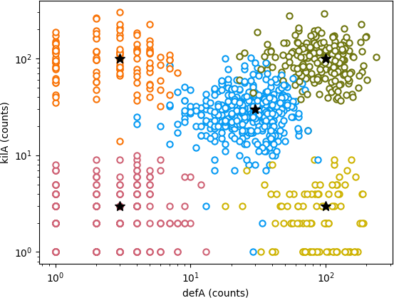 Figure 2: Another figure from Wiggins' notebook, showing the true
clustering of the 1000 cells.
Figure 2: Another figure from Wiggins' notebook, showing the true
clustering of the 1000 cells.
1. reproduce Wiggins' K-means result
Write a standard K-means clustering procedure. Use it to cluster Wiggins' data into K=5 clusters. Plot the results, similar to his figure. You should be able to reproduce a similarly bad result.
You'll want to run the K-means algorithm multiple times and choose the best. What is a good statistic for choosing the "best" solution for K-means? You should be able to reproduce Wiggins' "tot_sqdist" measure.
Why is K-means clustering producing this result, when there are clearly five distinct clusters in the data?
2. mixture negative binomial fitting
Now you're going to use what you've learned about mixture models, and about the negative binomial distribution for RNA-seq data.
Write an expectation maximization algorithm to fit a mixture negative binomial distribution to Wiggins' data, for Q=5 components in the mixture.
Assume there is a common dispersion \(\phi = 0.2\). This means that all you need to re-estimate in the EM algorithm are the means \(\mu\) and mixture coefficients \(\pi\) for each mixture component.
Like K-means, EM is a local optimizer, so you will want to run your EM algorithm from multiple initial conditions, and take the best one. What is an appropriate statistic for choosing the "best" fit?
What are the estimated mean expression levels of defA and kilA in the five cell types, and the relative proportions of each cell type in the 1000 cells?
Visualize your result in a plot similar to Wiggins'.
3. find a simple fix for K-means
Suggest a simple fix for the problem in applying a standard K-means clustering algorithm to Wiggins' single cell RNA-seq data. Implement the fix, re-run the K-means clustering, pick a "best" solution; report and visualize it.
allowed modules
Our list of allowed modules now includes NumPy, Matplotlib, Pandas, Seaborn, and SciPy's stats and special modules.
You'll probably want scipy.stats.nbinom.logpmf() for the log
probability mass function of the negative binomial, and
scipy.special.logsumexp() for summing probabilities that you're
storing as log probabilities. You might use Pandas for parsing
Wiggins' data table, though I didn't.
My imports, for example:
import numpy as np
import matplotlib.pyplot as plt

import scipy.stats   as stats               # for stats.nbinom.logpmf()
import scipy.special as special             # for special.logsumexp()

%matplotlib inline
turning in your work
Submit your Jupyter notebook page (a .ipynb file) to
the course Canvas page under the Assignments
tab.
Name your
file <LastName><FirstName>_<psetnumber>.ipynb; for example,
mine would be EddySean_09.ipynb.
We grade your psets as if they're lab reports. The quality of your text explanations of what you're doing (and why) are just as important as getting your code to work. We want to see you discuss both your analysis code and your biological interpretations.
Don't change the names of any of the input files you download, because the TFs (who are grading your notebook files) have those files in their working directory. Your notebook won't run if you change the input file names.
Remember to include a watermark command at the end of your notebook,
so we know what versions of modules you used. For example,
%load_ext watermark
%watermark -v -m -p jupyter,numpy,matplotlib,scipy
hints
-
The true cell type is noted in the data file, so you can check whether your clustering algorithms are working well. (It's sort of obvious where the five clusters are anyway, visually, so it's not like I'm giving much away.)
-
K-means (and fitting mixture models by EM) is prone to spurious local optima -- as you'll surely see. A lot of the art is in choosing initial conditions wisely. You may want to try some different strategies.
-
The mixture modeling EM algorithm will be eerily parallel to your K-means algorithm (cough that's the point of the pset cough cough). The expectation step, in which you calculate the posterior probability that each data point \(i\) belongs to component \(q\), is analogous to the K-means step of assigning a data point \(i\) to the current closest centroid \(q\). The maximization step, in which you re-estimate the \(\mu\) parameters given the posterior-weighted points, corresponds to the K-means step of estimating new centroids from the mean of their assigned points.
-
A big hint on part (3): consider how K-means assigns its points to centroids, versus how Wiggins plotted the axes when he visualized these data.
-
K-means is also prone to artifacts when the variances of the clusters are different, or when the variances aren't uniform in the different directions (dimensions), because it implicitly assumes spherical Gaussian distributions of equal variance. I decided against fitting the NB dispersion parameters for this pset -- which would be easy enough to do by "method of moment" fitting, though a moderate pain by maximum likelihood, as it turns out.
-
You locate the script Wiggins used to read his data file and produce Figure 2. This might help you avoid some of the routine hassles of parsing input and producing output, and focus on the good bit (K-means and EM fitting of a mixture model).
take-home lessons
- On the one hand, I'm using the very intuitive K-means algorithm to illustrate how an EM algorithm works. On the other hand, I'm using EM fitting of a statistical mixture model to illustrate how K-means is a simplified case of mixture modeling that makes strong implicit assumptions.