Information theory in biology

Notes by Jenya Belousova (2024)

Entropy

As we remember from the lecture, Shannon entropy equation looks like this:

$$ H(x) = \sum_x p(x) \log_2 \frac{1}{p(x)} $$

This is the average encoding length required per symbol in a given sequence. Now let us look at MSA. MSA reduces our uncertainty about each position, so we can introduce the entropy of a column c in the alignment:

$$ H(c) = \sum_i p(i) \log_2 \frac{1}{p(i)} $$

where i is a nucleotide. This formula allows us to create entropic profiles for MSA of biopolymer: simply a plot of entropy in each position. For example, in Adami C., 2004 we find some analysis with entropic profiles. Here is an entropic profile for tRNA from E. coli:

Notably, nucleotides forming hydrogen bonds in the secondary structure (which means that they are crucial for this molecule) are not necessarily conserved in the cours of evolution. It is complementary pair what matters, and not always a specific nucleotide.

And what about proteins? Our theory allows us to consider the alphabet of 20 amino acids instead of 4 nucleotides and apply all the same analysis to a protein MSA. Here is a curious application of information theory approach to the study of drug resistance. The same author constructed an entropic profile of the HIV-1 protease, which is quite distinguishable from tRNA profile.

Entropic profile of a protein visualizes positions with high conservation as well as polymorphic positions. The above profile was constructed for viruses exposed to a drug, and we can see two highly conserved regions there, while viruses not exposed to the treatment have three coserved regions in their genomes. It is believed that the polymorphisms emerging during the treatment contribute to resistance mutations. However, from just a profile like this one it is still hard to say which polymorphisms are responsible for drug resistance. In fact, there is a better way to use entropic profiles to gain such information. Here is the change of an entropic profile for the same protease after six months of treatment with high doses of saquinavir.

On this plot there are actually two types of changes: mutations in regions that were previously conserved (true resistance mutations), and changes in the substitution pattern on sites that were previously polymorphic. Negative peaks correspond to the reduced polymorfic variance in those sites.

Some of the resistance mutations actually appear in pairs on the entropic profiles, because they depend on each other. But there is a much better metric for tracking functional links between monomers - mutual information.

Mutual information calculation

Getting closer to the pset, let us have a look at the example of mutual information calculation. The formula for mutual information:

$$ M_{ij} = \sum_{a,b} p_{ij}(a,b) \log_2 \frac{p_{ij}(a,b)}{p_i(a) p_j(b)} $$

Here is the toy example of its application:

In this toy example we have a lot of cases where we cannot compute the logarithm because of 0 probability. (However, in actual alignments these cases will be much less common because of the significant alignment depth.) One way to deal with this uncertainty - addition of pseudocounts. You sort of add one artificial combination of each type in positions 1 and 8, and as a result $p_{ij}(a,b)$ will be very close, but not equal, to 0, and instead of uncertainty you will get a very low value, which will not change the $M_{ij}$ much.

Mutual information distribution: actual and randomized

After your python function has computed $M_{ij}$ for each pair of columns, you get a distribution of 2556 $M_{ij}$ values for the actual alignment. Pset requires to plot this distribution, so let us show it schematically (assuming we don't know yet how it actually will look like):

To obtain negative control we can perform a shuffling procedure and plot a fake $M_{ij}$ distribution. Survival function might help to justify your choice of a "significant" $M_{ij}$ threshold, so it is also required to be plotted.

Other applications of mutual information

Sometimes we are interested not in specific values of mutual information for particular positions of MSA, but rather more broadly in distribution of dependencies within a biomolecule. Another use of mutual information metric is to plot how it depends on the distance between monomers ($n$) in general. The authors in the work Ebeling & Frommel, 1998 performed such analysis for two proteins.

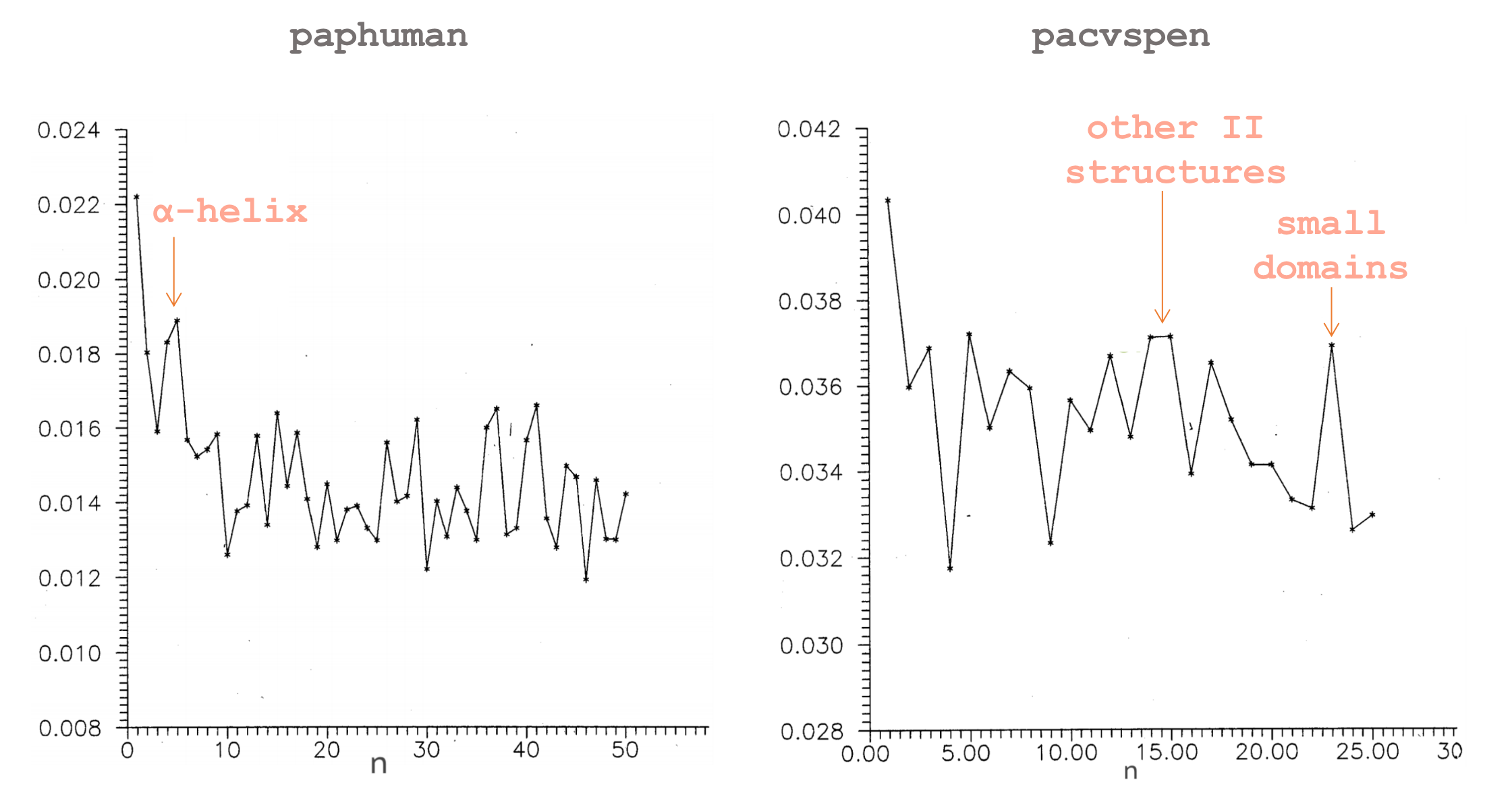
Paphuman has a well-pronounced peak around $n=4$. Indeed, apolipoproteins are $\alpha$-helix enriched and in $\alpha$-helices approximately every fourth amino acid interact with each other. Multifunctional enzyme pacsven has peaks around $n=15$ and $n=25$, which are the size of secondary structural elements and small domains, respectively.

This analysis allows us to draw some conclusions about protein 3D structure and, in some cases, even function by just looking at its sequence, which is quite impressive.

To the large extent we are surrounded by the world of evolving sequences, and not only biological. Same authors repeat this analysis for music written by different composers.

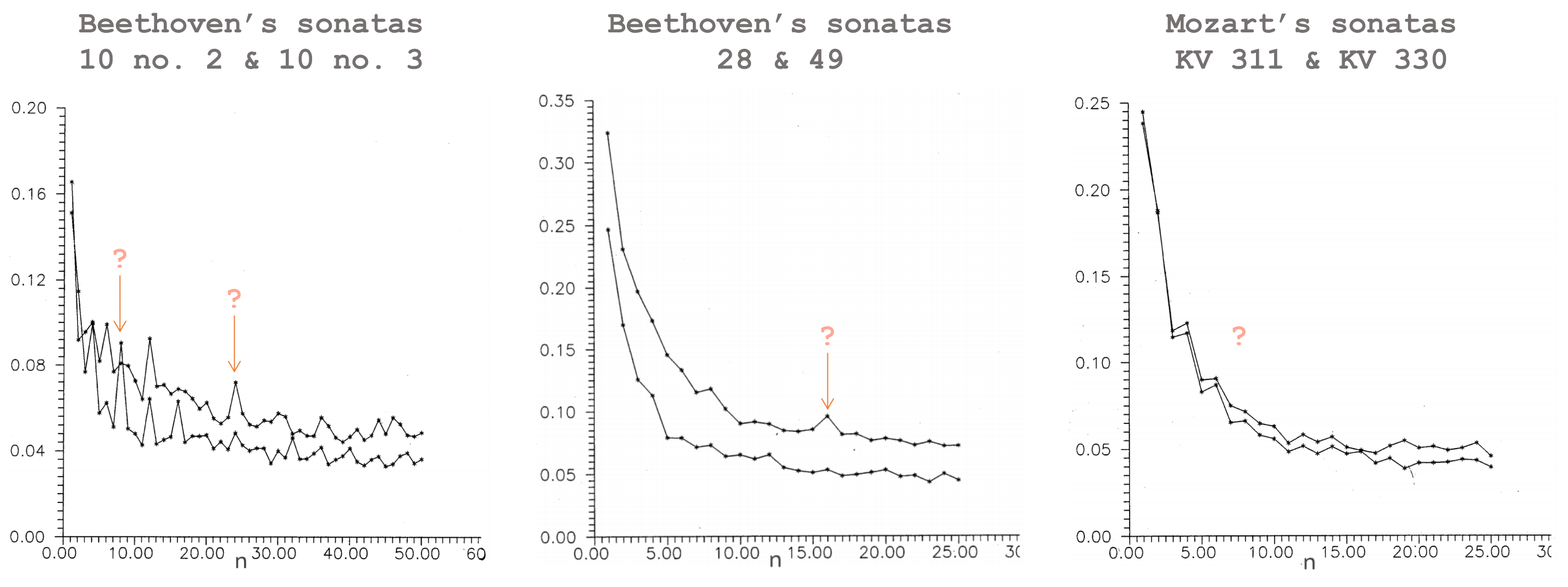
Since music mostly has an effect on the brain, it is hard to talk about any musical "phenotype" at the current state of development of neural sciences. But music is definitely well-structured and these plots might be a good way to capture these structures, even though we don't know how to describe them (yet).