week 05: Bayesian probabilistic inference
the eight-fold way
Eight points suffice to grasp the main practicalities of probabilistic inference.
1. random variables
A random variable is something that can take on a value. The value might be discrete (like "boy" or "girl", or a roll of a die 1..6) or it might be real-valued (like a real number \(x\) drawn from a Gaussian distribution). We'll denote random variables or events with capital letters, like \(X\). We'll denote values or outcomes with small letters, like \(x\).
When we say \(P(X)\) (the probability of random variable \(X\)), we are envisioning a set or array of values \(P(X=x)\), the probability that we could get each possible outcome \(x\).
Probabilities sum to one. If \(X\) has discrete outcomes \(x\), \(\sum_x P(X=x) = 1\). If \(X\) has continuous outcomes \(x\), \(\int_{-\infty}^{\infty} P(X=x) = 1\).
For example, suppose we have a fair die, and a loaded die. With the fair die, the probability of each outcome 1..6 is \(\frac{1}{6}\). With the loaded die, let's suppose that the probability of rolling a six is \(\frac{1}{2}\), and the probability of rolling anything else (1..5) is 0.1. We have a bag with fair dice and loaded dice in it. We pick a die out of the bag randomly and roll it. What's the probability of rolling 1, 2, ..., or 6? We have two random variables in this example: let's call \(D\) the outcome of whether we chose a fair or a loaded die, and \(R\) the outcome of our roll. \(D\) takes on values \(f\) or \(l\) (fair or loaded); \(R\) takes on values 1..6.
2. conditional probability
\(P(X \mid Y)\) is a conditional probability distribution: the probability that X takes on some value, given a particular value of \(Y\).
To put numbers to a discrete conditional probability distribution \(P(X \mid Y)\), envision a table with a row for each outcome of variable \(Y\), and a column for each outcome of variable \(X\). Each row sums to one: \(\sum_X P(X \mid Y) = 1\).
In our example, I told you \(P(R \mid D)\): the probability of rolling the possible outcomes 1..6, when you know whether the die is fair or loaded.
| roll R = | 1 | 2 | 3 | 4 | 5 | 6 |
|---|---|---|---|---|---|---|
| D = fair: | \(\frac{1}{6}\) | \(\frac{1}{6}\) | \(\frac{1}{6}\) | \(\frac{1}{6}\) | \(\frac{1}{6}\) | \(\frac{1}{6}\) |
| D = loaded: | 0.1 | 0.1 | 0.1 | 0.1 | 0.1 | 0.5 |
3. joint probability
\(P(X,Y)\) is a joint probability: the probability that X takes on some value and Y takes on some value.
Again, envision a table with a row (or column) for each variable \(Y\), and a column (or row) for each variable \(X\) -- but now the whole table sums to one, \(\sum_{XY} P(X,Y) = 1\).
For instance, we might want to know the probability that we chose a loaded die and we rolled a six. You don't know the joint distribution yet in our example, because I haven't given you enough information.
4. relationship between conditional and joint probability
The joint probability that \(X\) and \(Y\) both happen is the probability that \(Y\) happens, then \(X\) happens given \(Y\):
Also, conversely, because we're not talking about causality (with a direction), only about statistical dependency:
so:
So for our example, let's suppose that the probability of choosing a fair die from the bag is 0.9, and the probability of choosing a loaded one is 0.1. That's \(P(D)\). Now we can calculate the joint probability distribution \(P(R,D)\) as \(P(R \mid D) P(D)\).
| roll R = | 1 | 2 | 3 | 4 | 5 | 6 |
|---|---|---|---|---|---|---|
| D = fair: | \(\frac{9}{60}\) | \(\frac{9}{60}\) | \(\frac{9}{60}\) | \(\frac{9}{60}\) | \(\frac{9}{60}\) | \(\frac{9}{60}\) |
| D = loaded: | 0.01 | 0.01 | 0.01 | 0.01 | 0.01 | 0.05 |
If you have additional random variables in play, they stay where they are on the left or right side of the \(\mid\). For example, if the joint probability of \(X,Y\) were conditional on \(Z\):
Or, if I start from the joint probability \(P(X,Y,Z)\):
5. marginalization
If we have a joint distribution like \(P(X,Y)\), we can "get rid" of one of the variables \(X\) or \(Y\) by summing it out:
It's called marginalization because, imagine a 2-D table with rows for Y's values and columns for X's values. Each entry in the table is \(P(X,Y)\) for two specific values \(x,y\). If you sum across the columns to the right margin, your row sums give you \(P(Y)\). If you sum down the rows to the bottom margin of the table, your column sums give you \(P(X)\). When we obtain a distribution \(P(X)\) by marginalizing \(P(X,Y)\), we say \(P(X)\) is the marginal distribution of \(X\).
In our example, we can marginalize our joint probability matrix:
| roll R = | 1 | 2 | 3 | 4 | 5 | 6 | P(D) |
|---|---|---|---|---|---|---|---|
| D = fair: | \(\frac{9}{60}\) | \(\frac{9}{60}\) | \(\frac{9}{60}\) | \(\frac{9}{60}\) | \(\frac{9}{60}\) | \(\frac{9}{60}\) | 0.9 |
| D = loaded: | 0.01 | 0.01 | 0.01 | 0.01 | 0.01 | 0.05 | 0.1 |
| P(R): | 0.16 | 0.16 | 0.16 | 0.16 | 0.16 | 0.20 |
Now we have the marginal distribution \(P(R)\). This is the probability that you're going to observe a specific roll of 1..6, if you don't know what kind of die you pulled out of the bag. You've marginalized over your uncertainty of an unknown variable \(Y\). Because sometimes you pull a loaded die out of the bag, the probability that you're going to roll a six is slightly higher than \(\frac{1}{6}\).
If I have additional random variables in play, again they stay where they are. Thus:
and:
6. independence
Two random variables \(X\) and \(Y\) are independent if:
which necessarily also means:
In our example, the outcome of a die roll \(R\) is not independent of the die type \(D\), of course. However, if I chose a die and rolled it \(N\) times, we can assume the individual rolls are independent, and the joint probability of those rolls could be factored into a product of their individual probabilities:
In probability modeling, we will often use independence assumptions to break some big joint probability distribution down into a smaller set of terms, to reduce the number of parameters in our models. The most careful way to invoke an independence assumption is in two steps: first write the joint probability out as a product of conditional probabilities, then specify which conditioning variables are going to be dropped. For example, we can write \(P(X,Y,Z)\) as:
Then state, "and now I will assume Y is independent of Z, so:"
It's possible to have a situation where \(X\) is dependent on \(Y\) in \(P(X \mid Y)\), but when a variable \(Z\) is introduced, \(P(X \mid Y,Z) = P(X \mid Z)\). In this case we say that \(X\) is conditionally independent of \(Y\) given \(Z\). For example, \(Y\) could cause \(Z\), and \(Z\) could cause \(X\); \(Y\)'s effect on \(X\) is entirely through \(Z\). This starts to get at ideas from Bayesian networks, a class of methods that give us tools for manipulating conditional dependencies and doing inference in complicated networks.
7. Bayes' theorem
We're allowed to apply the above rules repeatedly, algebraically, to manipulate probabilities. Suppose we know \(P(X \mid Y)\) but we want to know \(P(Y \mid X)\). From the definition of conditional probability we can obtain:
and from the definition of marginalization we know:
Congratulations, you've just derived and proven Bayes' theorem:
If you assume that \(P(Y)\) is a constant (a uniform prior) it cancels out, and you recognize Laplace's inverse probability calculation from week 02.
8. why Bayes' theorem is a big deal
If we were just talking about \(X\) and \(Y\) as random variables, Bayes' theorem would be trivial. I mean, there you go, we just derived it in a couple of lines.
Things get interesting when we talk about observed data \(D\) and a hypothesis \(H\):
The probability of our hypothesis, given the observed data, is proportional to the probability of the data given the hypothesis, times the probability of the hypothesis before you saw any data. The denominator, the normalization factor, is \(P(D)\): the probability of the data summed over all possible hypotheses.
\(P(D \mid H)\), the probability of the data, is usually the easiest bit. This is often called the likelihood. (It's the probability of the data \(D\); it's the likelihood of the model \(H\).)
\(P(H)\) is the prior.
\(P(D)\) is sometimes called the evidence: the marginal probability of the data, summed over all the possible hypotheses that could've generated it.
\(P(H \mid D)\) is called the posterior probability of \(H\).
Bayes' theorem looks like it's telling us how to do science. Bayes' theorem gives us a principled way to calculate the posterior probability of a hypothesis \(H\), given data \(D\) that we've observed.
Well, hold on -- maybe, but we do have some problems. Where do we get \(P(H)\) from, if it's supposed to be a probability of something before any data have arrived? We may have to make a subjective assumption about it, like saying we assume a uniform prior: assume that all hypotheses \(H\) are equiprobable before the data arrive.
Second, how do we enumerate all possible hypotheses \(H\)? Sometimes we'll be in a hypothesis test situation of explicitly comparing one hypothesis against another, but in general, there's always more we could come up with.
And third, perhaps most worrying of all, what does it mean to talk about the probability of a hypothesis? You might well argue that a hypothesis is either true or false; it's not a repeatable experiment that you're sampling observations from and getting a frequency.
A key feature of Bayesian inference is that we treat probability as a degree of belief, not just as a sampling frequency. This difference is the principal difference between two statistical philosophies, "Bayesians" and "frequentists".
derivation of the i.i.d. and position-specific motif models
Recall from week 02 that for many common sequence analysis problems, we want to express the probability of a sequence \(x_1..x_L\) of length \(L\) given some probability models. For example, we might be interested in a binary classification problem where we're trying to distinguish sequences that look more like they came from one source versus another, and we approach the problem by making probability models for the distribution of sequences we expect from each source.
We saw a couple of different ways to factorize \(P(x_1..x_L \mid \theta\)) to have a parameterized model \(\theta\) where the number of parameters is reasonable.
We saw that an i.i.d. model of DNA sequences of length \(L\) assumes that each residue is independently generated from the same distribution over A|C|G|T, so it only has four parameters:
We also saw that an ungapped position-specific motif model of length \(L\) assumes that each position \(i\) has distinct preferences \(p_i(a)\) for each nucleotide \(a\), so it has \(4L\) parameters:
There models seem pretty obvious, but let's have a more formal look at their derivation under the rules of the eight-fold way.
Suppose (for sake of example) we have a sequence of six residues, \(UVWXYZ\), where each symbol represents a random variable that takes a value a/c/g/t. We want to express a joint probability \(P(UVWXYZ)\). We can exactly factor that joint probability into a series of conditional probabilities like so:
All exact, so far; no approximation. All we did was converted joint probabilities to conditional probabilities, repeatedly.
Now we can look at terms like, e.g., \(P(Z \mid UVWXY)\) and make independence assumptions. \(Z\) depends on \(U,V,W,X,Y\)? Well, let's assume it doesn't. We can go through each term and remove one, some, or all of the dependencies, and each time we do, that corresponds to stating an assumption that the nucleotide at \(Z\) doesn't depend on the nucleotide at the variable (position) we remove. Or at least, doesn't depend enough that we care, for the purposes of making a model, given the cost/benefit tradeoff of balancing the number of free parameters we need to estimate, versus what we gain from a more exact model.
The most extreme and simple thing we could assume is that \(Z\) doesn't depend on any other position: \(P(Z \mid UVWXY) \simeq P(Z)\). Make that assumption all the way down the chain and we have \(P(UVWXYZ) = P(U) P(V) P(W) P(X) P(Y) P(Z)\).
We could still have different distributions at the six positions. Maybe position \(U\) is often an A, position \(V\) is usually C or G, position \(W\) is equiprobably any of the four, and so on. If we allow each of the six random variables (positions) to have its own distribution, we have the position-specific motif model, with \(4L\) parameters.
But to simplify our model still more, we could state a further assumption that each of the six positions is drawn from the same nucleotide frequency distribution \(p(a)\) -- and that identically distributed assumption, on top of the independence assumptions, gets us to the i.i.d. model.
Markov models
Now let's move on to another common kind of probability model for sequences: Markov models.
Suppose we're ok with the identically distributed assumption -- we're not trying to capture position-specific statistical information (like in one particular conserved DNA sequence motif), we're trying to capture overall statistical properties and biases in a DNA sequence. But suppose that complete independence is an assumption that seems too strong.
For example, in coding sequences, individual bases aren't independent. They come in triplets because of the genetic code. Can we capture this dependence? We could try to factor a sequence of length \(L\) in terms of conditional probabilities of triplets (codons), followed by an independence assumption that codons are statistically independent, i.e.:
But this is a pretty specialized model that depends on the fact that there's a reading frame. We know exactly where to break the sequence into triplets. What if we have a problem where there's no frame?
For example, many eukaryotic genome sequences show a strong depletion of CG dinucleotides. If you count up mononucleotide and dinucleotide frequencies, you see that \(p(cg) << p(c)p(g)\). If we want to capture the fact that G is disfavored if the previous nucleotide was a C, we need something more than just an i.i.d. model. (And C is disfavored after a G, because of the other strand; the reverse complement of CG is GC.) Biologists refer to this as CpG bias, where the p in CpG indicates the phosphodiester linkage along a DNA strand -- we talk about CG composition so much in other contexts, we say CpG to keep it straight that we're talking about adjacent nucleotides.
If you tried to make a model that takes CpG bias into account, you might think you could do something with multiplying dinucleotide frequencies together, but probability algebra doesn't work that way.
So let's back up. Let's go all the way back to:
Dinucleotide composition bias means that we're not going to assume that \(Z\) is independent of its neighbor \(Y\), but we're still going to drop the rest:
If we make the identically distributed assumption, that the same dinucleotide bias holds everywhere in the sequence, then we can get to a general form:
We have two kinds of parameters. The main parameters are the \(p(b \mid a)\) parameters for the probability that nucleotide \(b\) follows \(a\). We also need to get the chain started somehow, so we need \(p(a)\) for the nucleotide probabilities at the first position.
K-th order Markov models
What we've just derived is called a first order Markov chain. In general, when someone says Markov model, they're talking about a model where they assume that the identity of position \(i\) depends on one or more previous positions \(i-1\), etc.
This generalizes to higher order Markov models. A 2nd order Markov chain would have terms \(p(c \mid a,b)\) and initial probabilities \(P(a,b)\). 3rd order would have \(p(d \mid a,b,c)\) and \(P(a,b,c)\). In general, for a \(K\)-th order Markov model:
derivation of log-likelihood ratio (LLR) scores
We also talked in week 02 about using LLR scores when we're doing a binary classification problem, where we can express our two competing hypotheses as probability models:
For example, we've seen LLR scores for individual residues in an alignment scoring system, where \(H_1\) states that two aligned residues \((a,b)\) come from a non-independent joint distribution \(p(a,b)\) because they're homologous (evolutionarily related), versus a null hypothesis \(H_2\) that states that they're independent, \(f(a) f(b)\).
Let's now see why LLR scores are justified. Bayes tells us that what we're really interested in is the posterior probability \(P(H_1 \mid x)\), if we're interested in inferring our degree of belief that observed sequence \(x\) is assigned to hypothesis \(H_1\).
So, starting from Bayes' theorem, dividing through first by \(P(H_1)\) in both numerator and denominator, then by \(P(x \mid H_2)\):
This is showing us that we can rearrange the posterior probability in terms of an ratio \(\frac{P(x \mid H_1)}{P(x \mid H_2)}\) that we can calculate, and a prior ratio \(\frac{P(H_2)}{P(H_1)}\) that we will also need to figure out what to do with.
Suppose we go ahead and define an LLR score \(\sigma(x)\). Then:
You might recognize this as a sigmoid function \(f(\sigma(x)) = \frac{e^{\sigma(x)}} {e^{\sigma(x)} + c}\) for a constant \(c = \frac{P(H_2)}{P(H_1)}\). For high scores, it asymptotically approaches 1; for low scores, it approaches 0; and it rises through 0.5 at \(\sigma(x) = \log \frac{P(H_2)}{P(H_1)}\). If the two models are a priori equiprobable, the sigmoid curve is centered with its midpoint at \(\sigma(x) = 0\). That is, an LLR score of 0 means that the two models are a posteriori equiprobable.
The log of the prior probability ratio acts as a constant offset on the score. If \(H_2\) is a priori more probable, then \(\log \frac{P(H_2)}{P(H_1)}\) is positive -- the sigmoid curve shifts to the right, signifying that it takes more LLR score to convince you that the data favor \(H_1\), even though \(H_1\) was less probable a priori.
There might be problems where the prior probabilities are known. For example, the fair vs. loaded die problem is an example, where I'm given the prior probability of choosing a fair vs. loaded, before I observe data (a roll) from that die. The pset this week is another example, where we're told that the probability of a Streptomyces phage read is 0.1% and the probability of a Microbacterium phage read is 99.9%, before we observe a sequence conditional on that model. In such cases, we could directly and correctly calculate the Bayesian posterior we need.
But for many problems, the priors aren't known. In such cases, the LLR is about the best probability-based score we can use, and we have to keep in mind that we don't know the offset in that sigmoid plot for how the LLR relates to the posterior probability of our classification.
Sometimes \(\frac{P(x \mid H_1)}{P(x \mid H_2)}\) (without the log) is called the Bayes factor.
evaluating classification performance: ROC plots
Suppose we've developed a score for a binary classifier -- whether it's an LLR score, or even if it's something arbitrary. We could choose to set a score threshold \(t\) such that if \(\sigma(x) > t\) we assign it to class \(H_1\), and otherwise we assign it to \(H_2\). Suppose we're looking for a particular class of interesting things ("positives", class \(H_1\)) against a background of uninteresting things ("negatives", class \(H_2\)).
Indeed \(H_2\) might be so boring and uninteresting that it's our model of "nothing is going on with \(x\) except random chance": it is a null hypothesis.
Where should we set the threshold \(t\), to achieve the best results in discriminating positives from negatives?
There is no single answer to this question, because it depends on whether we care more about not missing any positives, or about not making a mistake of misclassifying a negative as a positive.
Imagine a little 2x2 matrix of the truth versus our classification:
- true positive (TP) is when we call \(x\) positive and it is one;
- true negative (TN) is when we call \(x\) negative and it is;
- false positive (FP) is when we call \(x\) positive and it's really noise
- false negative (FN) is when we call \(x\) negative and it's really signal
From these counts, we can calculate:
"Sensitivity" goes by other names, including the true positive rate, or recall.
1 - specificity is also called the false positive rate.
If we set the score threshold lower (less stringent), we classify more stuff positive: our sensitivity increases, but our specificity drops. We can ultimately achieve 100% sensitivity, but 0% specificity, by calling everything a positive. If we set the threshold higher, the sensitivity drops, but our specificity increases; we achieve 100% specificity, but 0% sensitivity, by calling everything a negative.
A plot of sensitivity versus false positive rate (both from 0 to 1.0) for all possible choices of threshold is called a receiver operating characteristic plot (ROC plot). The name "receiver operating characteristic" is a historical artifact, as you might guess. It's military jargon that arose in WWII for radar receivers distinguishing blips as enemy vs. friendly aircraft. Correct friend/foe classification is a pretty important operating characteristic for a military radar receiver. A perfect ROC plot leaps immediately to 100% sensitivity at 0% FPR. Random guessing gives you a diagonal line.
a caveat to ROC plots
When you're in a situation of detecting a small number of positives against a background of a large number of negatives -- a needle in the haystack problem, common in genome-scale biological data analysis -- a ROC plot can give you a misleading sense of the accuracy of a classification procedure. The number of false positives you detect will scale with the number of negatives you screen. You can have a procedure with a high specificity that still detects an unacceptable number of false positives, if the positives you're looking for are rare.
For this reason, there's two other common statistics that people calculate, which take into account the relative frequency of positives versus negatives:
Of the set of things that you classify as positive, PPV is the fraction that you're right about, and FDR is the fraction that you're wrong about. Notice that FDR = 1 - PPV.
For the reason above, it is quite possible to have a low false positive rate but an unacceptably high FDR.
The wikipedia page on sensitivity and specificity gives chapter and verse on these concepts and more.
bonus section: Occams razor
Occam's razor tells us to favor simpler hypotheses. But a more complex model, with more free parameters, will generally produce a better fit to the observed data. Imagine fitting a curve to some data points. As we allow more parameters in our curve, we eventually fit the data points exactly, even if we're just fitting noise. How do we decide when adding more parameters to a model is justified by the data? A remarkable and beautiful feature of Bayesian inference is that an automatic Occam's razor appears in the equations.
Imagine a trick coin factory that produces biased coins, such that any given coin can have any probability \(p\) of flipping heads from 0 to 1, uniformly distributed. I give you a coin, and I tell you there's a 50:50 chance that it's a fair coin versus a trick coin. You flip the coin 100 times, and you observe \(h\) heads. Now I'm going to offer you a bet on whether I gave you a fair or a trick coin. Can you calculate fair betting odds, given your observation of \(h\) heads out of 100 flips?
Making a maximum likelihood estimate of the coin's parametric (i.e. true, unknown) \(p\) is unhelpful to you. The "trick coin" hypothesis with a maximum likelihood estimate \(\hat{p} = \frac{h}{N}\), by definition, cannot give you a worse likelihood than the "fair coin" hypothesis that \(p=0.5\), because the trick coin hypothesis includes \(p=0.5\) itself as a possibility. Assuming a trick coin is guaranteed to give the best fit to the observed number of flips.
The trick coin factory is a simple example of having two hypotheses \(H_0\) and \(H_1\), where \(H_1\) is a more complex hypothesis with more free parameters (in this case, one versus zero). In particular, the trick coin factory is an example of a common situation called nested hypotheses, where \(H_0\) is a specific case of \(H_1\) -- the free parameter(s) of \(H_1\) can be set so that \(H_1 = H_0\). In this situation, \(H_1\) can never be a worse explanation for the data than \(H_0\), because \(H_1\) includes \(H_0\). If I fit \(H_1\) to the data by making a maximum likelihood estimate \(\hat{p}\), we know the simple hypothesis \(H_0\) cannot have a better likelihood; \(P(D \mid H_1, \hat{p}) \geq P(D \mid H_0)\). No Occam's razor here. Maximum likelihood fitting always favors more complex hypotheses.
Bayesian inference tells me that I'm supposed to compare \(P(\mathrm{data} \mid H_0)\) to \(P(\mathrm{data} \mid H_1)\), not to \(P(\mathrm{data} \mid H_1, \hat{p})\). The unknown value of \(p\) for \(H_1\) is a so-called nuisance parameter. I can't calculate a likelihood for \(H_1\) without \(p\), but I don't know what \(p\) is. Probabilistic inference tells me I have to integrate it out by marginalization:
(This calculation turns out to be a Beta integral, which we saw in passing in week 02. The first term \(P(\mathrm{data} \mid H_1, p)\) is just a binomial distribution again, but we would need introduce something called the Dirichlet distribution as a convenient way to parameterize \(P(p \mid H_1)\).)
Intuitively, here's what will happen. By varying \(p\), we can make \(H_1\) consistent with lots of different observed data -- any possible count \(h\) from 0 to 100. \(H_0\), with its fixed value \(p=0.5\), is only capable of explaining a narrow range of observed data. The likelihood of a hypothesis \(P(D \mid H)\) is a probability, so it must sum to one over all possible observed data. There's only so much probability to go around. A more complex hypothesis that's compatible with lots of different observed data must necessarily tend to assign lower probability to any given set of observations. A simpler hypothesis can commit more of its probability mass onto the narrower range of observations that it's compatible with.
Thus, an Occam's razor arises naturally. If a simpler hypothesis can explain the data well, it will tend to have a higher posterior probability, compared to a more flexible hypothesis. This doesn't happen if you make optimized point estimates for model parameters; it only happens if you integrate out the unknown parameters.
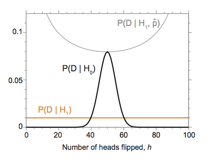
For example, if I calculate \(P(h \mid H_0)\) versus \(P(h \mid H_1)\) for the trick coin factory using a uniform Dirichlet prior, I get the result shown in the figure above. The trick coin hypothesis \(H_1\) can equally well explain any observation \(h=0..100\) (with \(P(h \mid H_1) = \frac{1}{101}\), unsurprisingly). The fair coin hypothesis \(H_0\) concentrates its probability mass around the expected \(h = 50\). Between about \(h=40\) and \(h=60\) heads, the fair coin hypothesis has a higher likelihood than the trick coin factory hypothesis.
(My example is contrived to match a famous figure from David J.C. MacKay's 1992 thesis.)
The plot also shows the likelihood \(P(h \mid H_1, \hat{p})\) for comparison, showing that the maximum likelihood fitted model \(H_1\) always dominates the simpler nested hypothesis \(H_0\).
Even if we observed exactly \(h=50\) heads, we can't be sure that the coin was fair, because trick coins can flip \(h=50\) heads too. The probability of observing \(h=50\) is 0.0796 for a fair coin, 0.0099 for a trick coin (averaged over uniform \(p\)). The odds are about 8:1 in favor of it being a fair coin, if we flip \(h=50\) heads with it. You can verify this yourself with a little Python script!
bonus extra example, with RNA-seq data
Suppose we've done a single cell RNA-seq experiment, where we've treated cells with a drug (or left them untreated), and we've measured how often (in how many single cells) genes A and B are on or off. Our data consist of counts of 2000 individual cells:
# Counts:
              T=no             T=yes
            B=ON  B=off      B=ON  B=off
   A=ON     180    80         10    360
   A=off    720    20         90    540
joint
The joint probabilities \(P(A,B,T)\) sums to one over everything. So normalize by dividing everything 2000 (the total # of cells):
# P(A,B,T)
              T=no              T=yes
            B=ON  B=off       B=ON  B=off
   A=ON     0.09   0.04       0.005  0.18
   A=off    0.36   0.01       0.045  0.27
marginal
Any marginal distribution is a sum of the joint probabilities over all the variables you don't care about, leaving the ones you do. For example, to get \(P(T)\), we sum over A,B: \(P(T) = \sum_{A,B} P(A,B,T)\), which leaves:
# P(T)
              T=no              T=yes
               0.5               0.5
conditional
A conditional distribution can be arrived at in a couple of different ways. One is to imagine building a separate joint probability table for each value of the condition. So we could for example focus just on the condition T=no; the subtable with T=no is:
# Counts, T=no
            B=ON  B=off
   A=ON     180    80
   A=off    720    20
and if we normalize that we get \(P(A,B \mid T=no)\):
# P(A,B | T=no)
            B=ON  B=off
   A=ON     0.18   0.08
   A=off    0.72   0.02
and we could do the same for the T=yes condition.
The other way is to manipulate things with probability calculus. Since \(P(A,B,T) = P(A,B \mid T) P(T)\), we can get a conditional probability distribution from the joint:
so the full table for \(P(A,B \mid T)\) is:
# P(A,B | T):
              T=no             T=yes
            B=ON  B=off      B=ON  B=off
   A=ON     0.18   0.08       0.01  0.36
   A=off    0.72   0.02       0.09  0.54
marginalizing a conditional probability
If we marginalize a conditional distribution, the conditioning stays as it was. For example, \(P(B \mid T) = \sum_A P(A,B \mid T)\), so:
# P(B | T):
               T=no           T=yes
            B=ON  B=off      B=ON  B=off
             0.9   0.1       0.1    0.9
and similarly we can get \(P(A \mid T) = \sum_B P(A,B \mid T)\):
# P(A | T):
               T=no           T=yes
   A=ON        0.26            0.37
   A=off       0.74            0.63
conditioning a conditional probability
Similarly when we make a new conditional distribution from a conditional, the thing we divide through by has the same condition. For example:
so the table for \(P(A \mid B,t)\) looks like:
# P(A | B,t):
               T=no           T=yes
            B=ON  B=off      B=ON  B=off
   A=ON     0.2    0.8        0.1  0.4
   A=off    0.8    0.2        0.9  0.6
independence
If A is independent of B, then \(P(A \mid T)\) = \(P(A \mid B, T\). Here that clearly isn't true. For example, the frequency of A+ cells among untreated cells is 0.26, but the frequency of A+ cells among B+ untreated cells is 0.2.
Simpsons paradox
If you think for a bit about what the numbers in this example are saying, you'll realize that there's something very counterintuitive going on.
Suppose I only look at the response of gene A to the treatment T: i.e. the distribution \(P(A \mid T)\). The fraction of cells positive for gene A clearly goes up after the cells are treated: from 0.26 to 0.37.
Now look at the response of gene A to treatment T when a cell is positive for gene B: i.e. \(P(A \mid B=on, T)\). The fraction B+ cells positive for gene A goes down by two-fold after treatment: from 0.2 to 0.1.
Now look at the B- cells: i.e. \(P(A \mid B=off, T)\). The fraction B- cells positive for gene A also goes down by two-fold after treatment: from 0.8 to 0.4.
So that means that if you hadn't measured B, you would've thought that the fraction of A+ cells was going up after treatment. But if you do measure B, in both B+ or B- cells, the fraction of A+ cells is going down after treatment.
This is Simpson's paradox.
One way to think about what's happening is that your intuition is (mistakenly) comparing \(P(A \mid T)\) to \(P(A \mid B,T)\) in your head as if they're directly comparable, and you can think of any difference you see as an effect on A. But \(P(A \mid T)\) is related to \(P(A \mid B,T)\) by marginalization:
so there's another way to affect \(P(A \mid T)\) "indirectly", which is through \(P(B \mid T)\). If A has a strong dependency on a hidden variable B, you'll get variation in A if you vary B. If your experiment varies something else (T), that's correlated with B, and you observe a change in A, you can't necessarily conclude that your T directly changed A; you might have only changed B.
For example, suppose B is really a cell type marker that has nothing directly to do with regulation of A, and that treatment causes B- cells to grow fast for some reason. Then after treatment, you've increased the fraction of B- cells in the population. If B- cells tend to express A at high level, and B+ cells express at low level, then the population-averaged level of A+ cells can look like it went up, even if the treatment actually downregulated A in both B+ and B- cells.
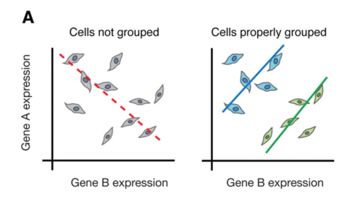 Figure 1A from
Trapnell (2015). Expression
levels of genes A and B
look anticorrelated (left), but you can get this result from
having two different cell types in the experiment
(blue and green, right), where gene A and B are positively
correlated in each individual type.
Figure 1A from
Trapnell (2015). Expression
levels of genes A and B
look anticorrelated (left), but you can get this result from
having two different cell types in the experiment
(blue and green, right), where gene A and B are positively
correlated in each individual type.
You can get Simpson's paradox effects with measured RNA-seq TPM values too. The nice figure above comes from 2015 review by Cole Trapnell, Defining cell types and states with single-cell genomics. Although Trapnell's article is about how single-cell RNA-seq experiments help avoid artifacts of bulk population averaging, the figure shows a plot of gene A and B levels in single cells, so the effect it illustrates can arise even in single cell data.
One famous example of Simpson's paradox occurred in a study of gender bias in PhD admissions at UC Berkeley. Statistics appeared to show that the chances of getting admitted to Berkeley are better if you're a man: 44% of men were admitted, but only 35% of women. But when the statistics were broken down by department, in each individual Berkeley department, the probability that a woman would be admitted was actually higher than the probability a man would be admitted. What was happening was that some departments have much lower admissions probabilities than others, and women were disproportionally applying to highly selective departments: the observed effect on \(P( \mathrm{admission} \mid \mathrm{gender})\) is through a confounding correlation \(P( \mathrm{department} \mid \mathrm{gender})\).
further reading
-
Sean Eddy, What is Bayesian statistics?, Nature Biotechnology, 2004.
-
David J.C. Mackay, Bayesian Interpolation, Neural Computation, 1992.