pset 02: the adventure of the hidden cloverleaf

Wiggins, one of the undergraduate senior thesis students in the lab who call themselves the Baker Street Irregulars, has found a 72 nucleotide DNA sequence that is conserved in hundreds of SEA-PHAGE.

Wiggins' guess is that the conserved sequence is a transfer RNA (tRNA) gene, and he wants to find evidence for or against this. Professor Holmes told him that since tRNAs have a distinctive base-paired secondary structure that resembles a cloverleaf, Wiggins should look for evidence supporting a consensus tRNA secondary structure for the conserved phage sequences.

That's not even really a joke. I'm referring to chemical and enzymatic RNA structure probing with chemicals like dimethylsulfate (DMS) (which methylates RNA at single-stranded A's and C's), and to enzymes like RNase V1 (which cleaves RNA primarily at base pairs). DMS is a toxic mutagen. RNase V1 comes from the venom of Caspian cobras. At one time in my work, V1 became hard to obtain because of a cobra shortage. Commercial sources are surely using the cloned/overexpressed RNase V1 gene these days.

Moriarty told Wiggins that he should make the RNA in vitro and do chemical and enzymatic structure probing with toxic mutagens and the venom of a Caspian cobra. Since Moriarty happens to keep a Caspian cobra at home, he offers to show Wiggins how to do these experiments.

The cloverleaf-like secondary structure of yeast phenylalanine tRNA. The GAA anticodon pairs with UUC and UUU Phe codons, allowing a third position "wobble pairing" of either C|U to position G34 of the anticodon. tRNAs typically have several post-transcriptionally modified bases, almost always including a thymine (T) and a pseudouridine (psi) in the TpsiCG loop and two dihydrouridines (D) in the D loop. Several other modifications more specific to yeast tRNA-Phe are shown in blue. The 75nt sequence of the mature tRNA includes a 3'CCA terminus that is added posttranscriptionally (orange). The tRNA gene sequence is 72nt long, exactly the length of Wiggins' phage DNA sequences. Source

Wiggins is hoping for an approach that's easier and less dangerous. He remembers you talking about an MCB112 lecture about using mutual information to detect pairwise covariation in RNA sequence alignments, as a way of detecting evolutionarily conserved RNA base pairing. He brings you a multiple alignment of 100 diverse examples of his conserved phage DNA sequence, and asks for your help.

Conveniently, knowing how you work, he also brings you a list of the consensus tRNA base pairs, already formatted for Python in pythonic 0-offset coords (off by one from the canonical 1..72 coordinate system that tRNAs are numbered in):

bp_list = [  (0, 70),  (1, 69),  (2, 68),  (3, 67),  (4, 66), (5, 65), (6, 64),   # 7bp acceptor stem
             (9, 23), (10, 22), (11, 21), (12, 20),                               # 4bp D stem
            (25, 41), (26, 40), (27, 39), (28, 38), (29, 37),                     # 5bp anticodon stem
            (47, 63), (48, 62), (49, 61), (50, 60), (51, 59) ]                    # 5bp T stem;  

(You'll use this list below. Trying to save you some tedium.)

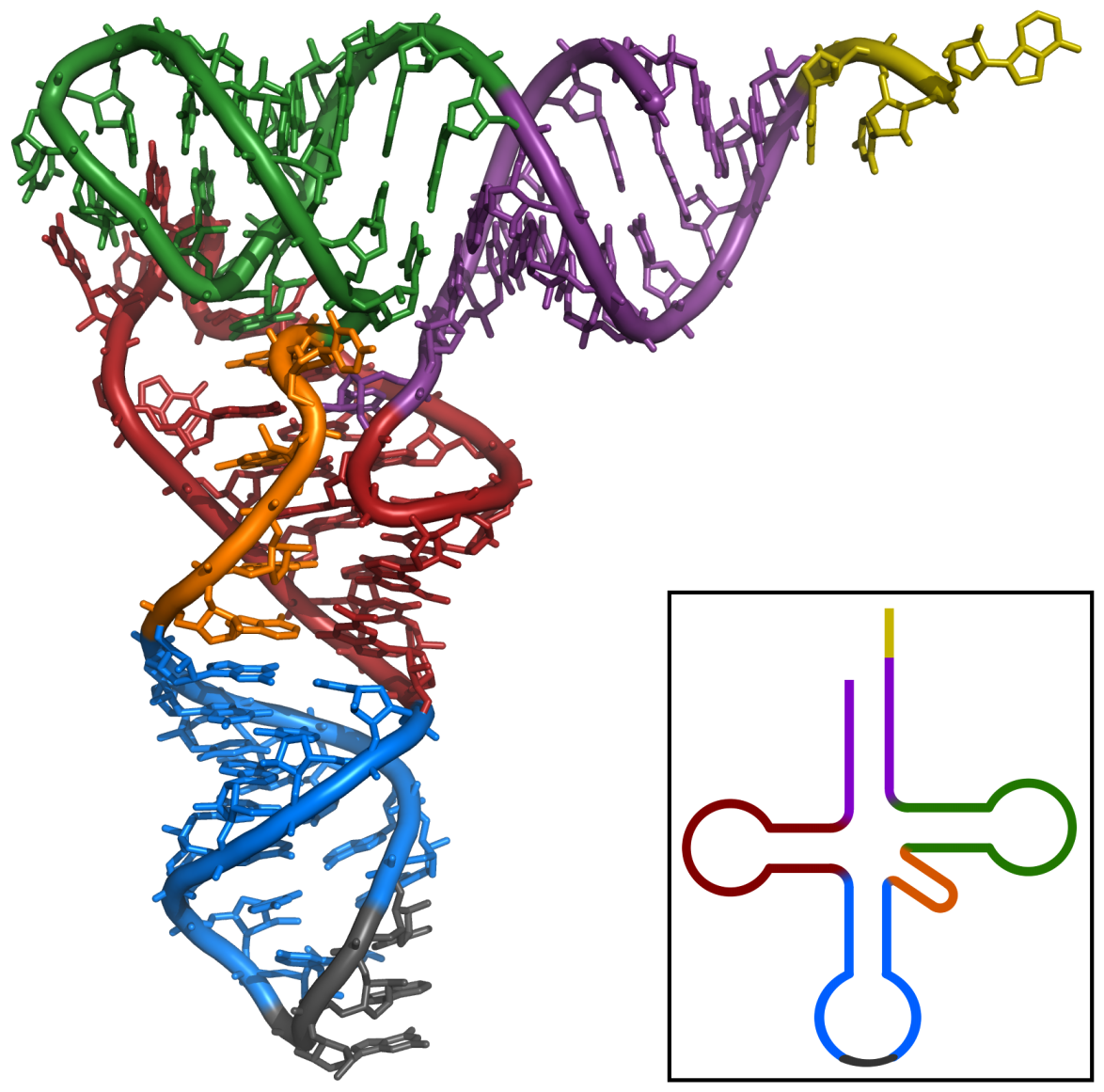The three-dimensional structure of yeast tRNA-Phe, with elements of the secondary structure color-coded to show where they are in the 3D structure. Source: PDB 1ehz

mutual information analysis

Download Wiggins' alignment from here (rna.msa). You can also use wget or curl to get it at the command line, for example with wget http://mcb112.org/w02/rna.msa.

The alignment is in a simple format. Each line has a sequence name, followed by the aligned DNA sequence. You notice that every sequence is exactly 72nt long: there are no gap characters in this "alignment". Wiggins explains that he used an ungapped position-specific weight matrix (PWM) to search the SEA-PHAGE genome sequence database for these examples. You tell him this wasn't the best way to identify homologous sequences, because of length variability due to insertions and deletions, but whatever. An ungapped multiple sequence alignment is easier to deal with.

We're discussing PWMs this week in class, though we're not using them yet.

1. Write Python code to read in the 100 aligned sequences, calculate mutual information between all pairs of columns \(i < j\), and plot these results in the upper \(i<j\) triangle of an LxL (72x72) heat map.

2. Explain the main features you see in this plot. Do you see evidence for the tRNA cloverleaf? What are some other things or patterns you see?

empirical statistical significance

Wiggins doesn't think Professor Holmes will be happy with just eyeballing a heatmap. He notes that the mutual information \(M_{ij}\) terms are positive whenever \(f_{ij} \neq f_i f_j\), and that's going to happen almost all the time just because of sampling noise. How high does an \(M_{ij}\) value need to be to be "significant"?

3. Devise a "null hypothesis" and write code to produce an alignment with the same primary sequence conservation statistics as the original MSA, but where pairwise correlations have been randomized.

That is, the singlet probabilities \(p_i(a)\) at each position of the randomized alignment are the same as the original, but the pairwise probabilities \(p_{ij}\) are now the independent product \(p_{ij}(a,b) = p_i(a) p_j(b)\). There are (at least) two ways to do this: either by a shuffling approach, or a generation/sampling approach. I am using the word "probability" carefully in the technical sense of the true parametric probability, as opposed to observed frequencies derived from counts. Observed frequencies \(f'_i(a)\) in a randomized alignment may not be exactly equal to the \(f_i(a)\) observed in the original if you use a generation/sampling approach instead of shuffling, and observed pairwise frequencies \(f'_{ij}\) in a randomized alignment will not be exactly equal to the independent product \(f'_i f'_j\) in either approach because of statistical noise. It's exactly that noise we want to characterize, to decide how high an \(M_{ij}\) mutual information needs to be before we consider it "significantly" higher than statistical noise.

4. Produce a set of many randomized MSAs and calculate mutual information values from them. Plot the distribution \(P(M_{ij} > t)\) versus varying threshold \(t\) for these negative control data. This is a so-called complementary cumulative distribution function, also known as a survival function. Also plot the distribution of the \(M_{ij}\) values from the actual rna.msa alignment. (There are 2556 of them: (L(L-1)/2).) Justify a choice of threshold \(t\) for calling an \(M_{ij}\) mutual information "significant".

5. Extract a list of all the putative consensus base pairs that satisfy your threshold. Compare your list to the list of consensus base pairs expected for tRNA. How many of the expected base pairs are supported by your mutual information analysis? If you see support for other pairs, give a possible explanation for them.

6. Does the mutual information analysis support Wiggins' hypothesis
that this conserved region encodes a tRNA?

hints and helpful guidance

How I broke this problem down myself (as hints, since we're still warming up in Python - though there are other good ways to do it too):

• a read_msa(msafile) function that parses the file into a list of sequence names, and a NumPy array called msa with nseq=100 rows and L=72 columns, where each value msa[s][i] is a character A|C|G|T in sequence \(s\) (0..nseq-1) at position \(i\) (0..L-1).

• a make_probmx(msa) function that takes that MSA and calculates the probabilities \(p_i(a)\) for residues indexed 0..3 (representing A..T). It stores these probabilities in a Lx4 numpy array pmx, with each row \(i\) being the distribution for position \(i\), so pmx[i][a] is \(p_i(a)\). It gets these probabilities as frequencies: first by counting observed residues, then normalizing each row. It returns pmx. (I made a separate function for this, instead of doing it within the mutual information function, because I played around looking at some other things in the primary sequence conservation pattern of the alignment.)

• a mutual_information(msa) function that takes the MSA and calculates mutual information values \(M_{ij}\) for all pairs of alignment columns \(i < j\). Recall that the equation for mutual information is:

where \(a,b\) iterate over all possible base pairs between columns \(i\) and \(j\). I call my make_probmx(msa) function to get the singlet probability terms I need for \(p_i(a)\) and \(p_j(b)\), and I calculate the pair probability terms \(p_{ij}(a,b)\) much like I did for the singlets, by collecting counts over all the sequences for columns \(i,j\) into a 4x4 counts matrix, then normalizing this to frequencies.

• a shuffle_msa(msa) function that takes the MSA and produces a randomized one using a shuffling approach.

• a sample_msa(msa) function that takes the MSA and produces a randomized one using a generation/sampling approach. (I did it both ways; you only need one.)

• for plotting the heat map, I use matplotlib's imshow(). (In my own research work I prefer using Seaborn heatmap, but we're being restricted to numpy and matplotlib imports for this pset.) Choose a good color map for your heatmap; you probably want a "sequential" one for this, and I'm a fan of the map called Blues, for example. You may also find that you want to use the vmin= and vmax= keyword arguments to imshow() to set the heatmap representation to the minimum and maximum possible mutual information value, so if you're comparing different datasets for some reason (like the shuffled datasets below), they're on the same scale.

• for plotting the two survival functions \(P(M_{ij} > t)\) for the original MSA vs. randomized negative control MSAs, I used matplotlib's ecdf() (empirical cumulative distribution function) with complementary=True to make it the complementary (survival plot) version.

allowed modules

NumPy and Matplotlib.

Set the %matplotlib inline "magic command" to get inline static figures from matplotlib in a Jupyter Notebook page.

import numpy as np
import matplotlib.pyplot as plt
%matplotlib inline

turning in your work

Submit your Jupyter notebook page (a .ipynb file) to the course Canvas page under the Assignments tab. Name your file <LastName><FirstName>_<psetnumber>.ipynb; for example, mine would be EddySean_02.ipynb.

We grade your psets as if they're lab reports. The quality of your text explanations of what you're doing (and why) are just as important as getting your code to work. We want to see you discuss both your analysis code and your biological interpretations.

Don't change the names of any of the input files you download, because the TFs (who are grading your notebook files) have those files in their working directory. Your notebook won't run if you change the input file names.

Remember to include a watermark command at the end of your notebook, so we know what module versions you used, in case we have to reproduce some bug exactly. For example,

%load_ext watermark
%watermark -v -m -p jupyter,numpy,matplotlib