Section 05: Intro to Probability
Notes Grace H. Zhang (2022), Colin Hemez (2021), Mary Richardson (2020), Gloria Ha (2019), Kate Shulgina (2018), and Jenya Belousova (2024)
The amazing gynandromorph
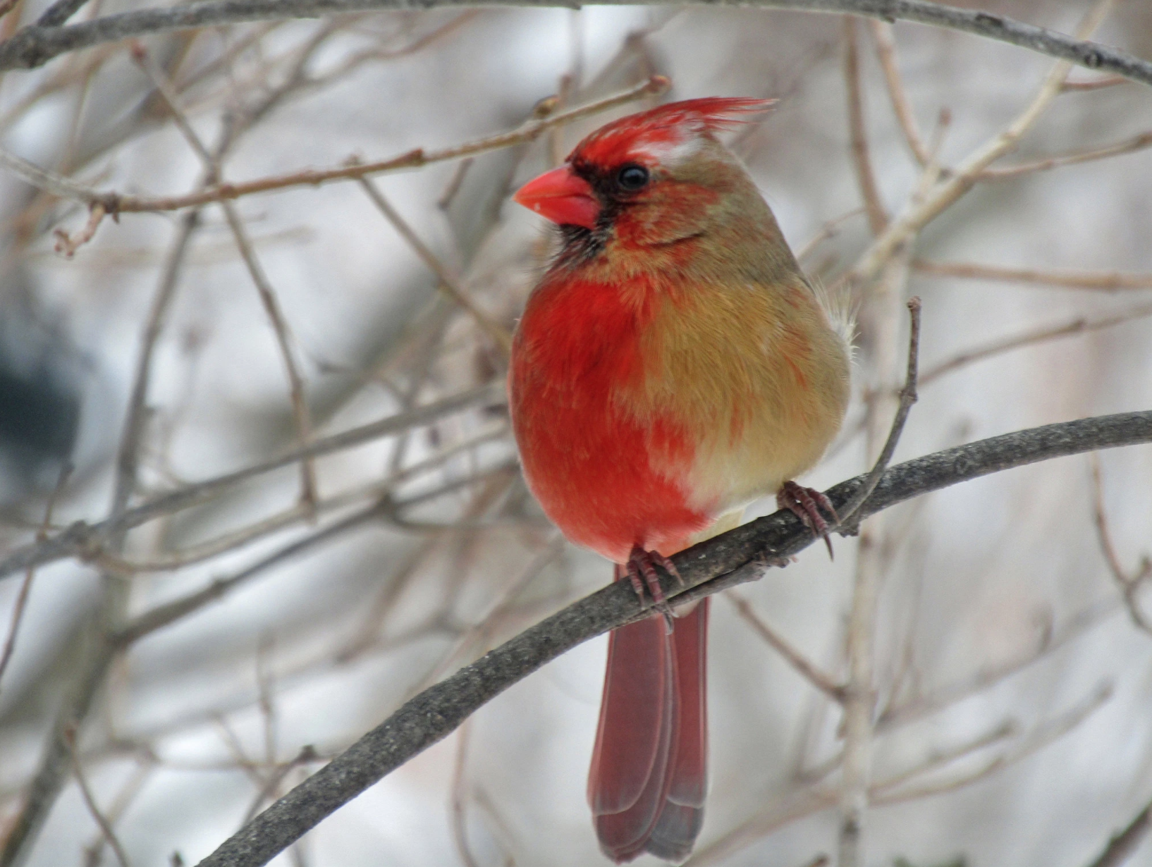
Here's one very special bird that was spotted in Pennsylvania in early 2019:

Image by Shirley Caldwell, https://www.nytimes.com/2019/02/09/science/cardinal-sex-gender.html
It's a gynandromorphic cardinal, an individual with both female and male characteristics. Gynandromorphism has been observed in vertebrates and invertebrates alike, but the case of the gynandromorphic cardinal is especially interesting (and visually stunning). Male cardinals are typically red, and female cardinals are typically gold, but there can exist considerable variability in plumage. This striking bilateral segmentation could not be due to gynandromorphism at all; it could also be the consequence of a somatic loss-of-function mutation that occurred very early in this bird's development.
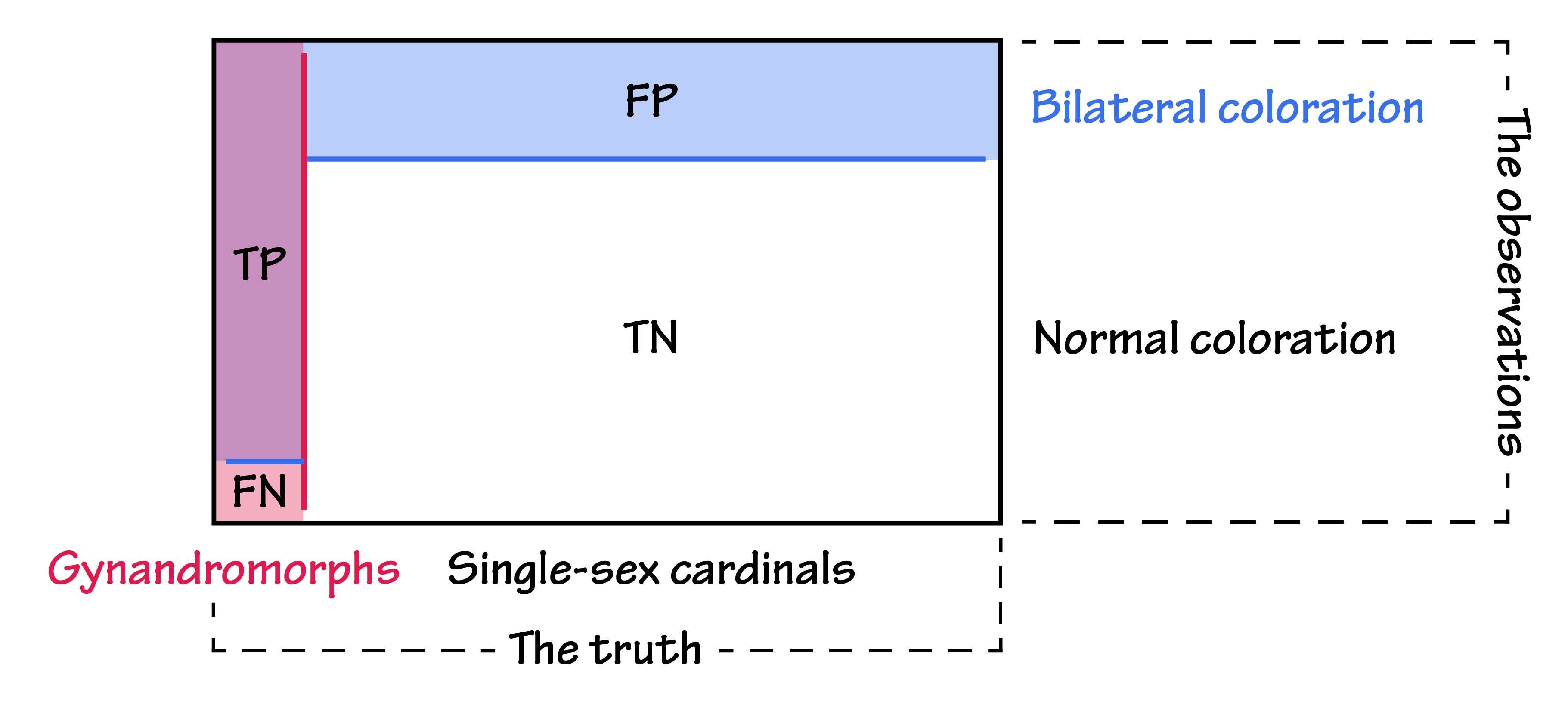
Gynandromorphic cardinals are rare, but very often have this remarkable plumage. Single-sex cardinals are very common, but can occasionally wear a coat of feathers that makes them look like a gynandromorph. So this raises a vexing statistical question: If you see one of these bicolor birds in the wild, what is the probability that it's a gynandromorph?
If we get Bayesian about it, we can figure this out. We'll cover this calculation in this section.
Markov models
(Another excuse to talk about birds)
In lecture, Sean introduced Markov models, which are very relevant for this week's pset. As discussed in class, Markov models are a way to calculate the probability of a sequence of events for which each event's probability only depends on the event(s) that came before it -- if you have a first order Markov model, the probability of an event depends only on the event that happened directly before, while if you have a second order Markov model, the probability of an event depends on the previous two events. The purpose of this section is to walk you through how you could implement your own Markov model (*cough cough* pset 05), explaining relevant terminology from the lectures and the pset along the way.
Let's make a toy Markov model to predict which species of bird is nearby based on the birdsongs we hear in the forest. We're in a forest that has two species of bird, sleek and fluffy, that each make songs composed of a mix of 'ree ree' calls and hiss-like 'ess ess' songs. If you're wondering how birds can make such a wide range of vocalizations like 'ess' and 'ree' and 'Hello!!!' , you can wonder at the formidable anatomic structure that is the syrinx.
You record the songs you hear in the forest, and encode the songs as a sequence of \(n\) 'ree' and 'ess' calls: 'rrssrssssr' or 'srsssrsr' for example. You want to know whether a bird is sleek or fluffy based on this pattern. You know that, over the course of a song, the next note that a bird will sing depends in part on the last few notes. So to account for this we will try modeling bird song using a third order Markov model, where the next note depends on the previous three notes.
Now let's set up our model!
Random variable
A random variable is a variable that takes on one of a defined set of values with some probability. Random variables are usually written as uppercase letters, and the values they assume are written lowercase. The set of values that a random variable can assume is called the sample space.
For our model, let \(X_i\) be the random variable of note \(i\). The note can be either 'ree' \((r)\) or 'ess' \((s)\), so the sample space for \(X_i\) is \(X_i \in {r,s}\). \(X_i\) will take on the value \(r\) if the note is 'ree' and \(s\) if the note is 'ess'. For example, if the first note in our song was 'ess', then we could denote event \(X_1=s\) as \(x_1\).
Joint probability
To calculate the probability of a given sequence of notes, we need to find the joint probability of all the notes in the sequence. For example, the probability of the sequence 'srs' is the probability that the first note in our sequence is 'ess' and the second note is 'ree' and the third note is 'ess'. Using our random variable notation from above, that is \(X_1=s\) and \(X_2=r\) and \(X_3=s\). This gives us the probability:
Or more generally:
Conditional probability
Say we want to find the conditional probability that the next note in our song is 'ess' given that the last three notes followed the sequence 'srs', which we represent as \(P(s|srs)\). It might feel more natural to think of the probability of the sequence 'srss', or \(P(srss)\). We can relate these two probabilities using the equation for conditional probability:
In other words, the probability of getting the sequence 'srss' can be written as the probability of getting 's' once you already have 'srs' multiplied by the probability of having 'srs' in the first place. We can rearrange this to solve for the conditional probability that we are interested in:
Or more generally:
Markov model
Now we're ready to define a third order Markov model where the next note of a song depends only on the previous three notes. To calculate the total probability of a song from this model, we need the two types of parameters we defined above:
- The initial probability \(P(x_1,x_2,x_3)\) is the joint probability of a particular sequence of three notes occurring. For example, the initial probability of a sequence starting with 'srs' is the probability of hearing 'ess', then 'ree', then 'ess'.
- The conditional probability \(P(x_i|x_{i-3},x_{i-2},x_{i-1})\) is the probability of observing the note \(x_i\) given the notes of the previous three notes. For example, the probability of 's' occurring after the sequence 'srs' is the probability of hearing 's' given that the previous three notes were 'srs'.
To find the total probability of a sequence using this model, we start by calculating the initial probability of the first three notes. For the sequence 'srsssrsr', this is \(P(srs)\). Next, for \(i=4\) we we want to know the probability of 's' after the sequence 'srs', which we write as \(P(s|srs)\). For \(i=5\), we want to know the probability of 's' after the sequence 'rss', or \(P(s|rss)\). And so on.
The total probability of a sequence from a 3rd order Markov model is then:
Kahoot break
That's a lot of explanation, let's take a break for a kahoot (live in class).
Training datasets
We have an equation for calculating the probability of a sequence from a third order Markov model... but how do we actually set the initial probability and conditional probability parameters? We need some data from which we can infer this knowledge. This is where a training dataset comes in. We have to train on a dataset of known songs for the sleek birds in order to calculate the probability that the new song we hear is from sleek.
To calculate the initial probability \(P(srs)\) for example, we can count how many times we see the sequence 'srs' in the training dataset and divide by the total number of 3-note sequences in the dataset. We can repeat this process for every possible 3-note sequence (3-mer, if you will) to find all initial probabilities.
Then to calculate the conditional probability, \(P(s|srs)\) for example, we can look back to the formula for conditional probability from above: \(P(s|srs) = \frac{P(srss)}{P(srs)}\) This shows us we need both \(P(srs)\) and \(P(srss)\) to get \(P(s|srs)\). We already know how to find \(P(srs)\) form the initial probabilities. Similarly, to find \(P(srss)\), we can count how many times we see the sequence 'srss' in the training dataset and divide by the total number of 4-note sequences in the dataset. We can again repeat this process for every possible 3-mer and 4-mer to find all conditional probabilities.
We can follow this process once to calculate our parameters for the sleek training dataset. Then we can repeat the process to calculate our parameters for the fluffy training dataset separately. Great – now our parameters are set!
Testing datasets
In the problem set, we are told to use half of the sequences as the training set, and half as the test set. The reason for this is we want to use data from known origins to train our model (get the probability parameters discussed above), and we also want to use data from known origins to test our model (see if we can figure out the bird species for a new song using our Markov model). But we DON'T want to use the same pieces of data to train and test the model! This is because we want our model to actually make predictions on data that it hasn't seen before (the test dataset). Depending on your data and model, you may use a larger or smaller fraction of the total dataset to train the model.
So how do we test the model? We want to see how well our model identifies the singer of our remaining recorded birdsongs. For each sequence in the test dataset, we should calculate the probability that the sequence came from sleek or fluffy. We do this by calculating the total probability of a sequence \(x = x_1, x_2,...,x_n\) using either the sleek parameters we trained or the fluffy parameters we trained:
- The probability of each test sequence \(x\) given the Markov model with sleek parameters \(H_0\) is \(P(x|H_0)\).
- The probability of each test sequence \(x\) given the Markov model with fluffy parameters \(H_1\) is \(P(x|H_1)\).
Log-odds score
We now know the probability that a specific sequence came from sleek or from fluffy. However, what we really want to know is how likely it is that the song came from sleek VERSUS fluffy (or the other way around, depending on what you consider a 'positive' – for this exercise we will consider sleek to be a positive result).
This is given by the log-odds score, which is the logarithm of the ratio of the probability of sequence \(x\) occurring under the third order Markov model with sleek parameters vs. with fluffy parameters:
Note that since this is a logarithm of a ratio, we can write it as the difference of two logs:
A note about log probabilities
If you remember from above, the probability \(P(x_1,x_2,...,x_n)\) is the product of numerous probabilities, so this can also be written as a sum of logarithms of probabilities. Why is this nice? Sometimes our probabilities are very small, and multiplying many small numbers together can give you underflow errors in Python (where the value gets rounded to zero because it's very very small). In future weeks, this will become super important!
Here, we are able to take the log because the probabilities we're dealing with are all positive – you can have trouble if you encounter probabilities of 0, so you add a small pseudocount as a positive offset inside the log.
Model performance
Now that we have an idea of how to construct a Markov model, how do we actually assess its performance? How do we know if our third order Markov model is actually any good at discriminating birdsongs from sleek and fluffy that we hear in the forest?
Score threshold
First off, we have a log-odds score for every sequence in our test dataset. How do we determine which songs are actually from sleek and which ones are from fluffy? We need to define a score threshold or cutoff – any sequence with a log-odds score above the threshold is from sleek and anything below it is from fluffy. Luckily we know the true species assignment of every song in our test dataset.
For any threshold that we set, there will be a corresponding number of:
- true positives (TP): sleek songs that are identified as sleek
- true negatives (TN): fluffy songs that are identified as fluffy
- false positives (FP): * fluffy songs that are identified as * sleek
- false negatives (FN): * sleek songs that are identified as * fluffy
We can calculate these values for a range of thresholds (say, the range of log-odds scores we get across the test dataset), and see how well we do at distinguishing the species. There are many metrics that combine TP, TN, FP, FN that you can consider when setting a threshold, and the pset mentions a few.
Confusion matrix
A common way to represent the TP, TN, FP, FN values for a given model is a confusion matrix. This is an awful name for a table containing these values. For example:
| Actual | Actual | ||
|---|---|---|---|
| sleek | fluffy | ||
| Predicted | sleek | TP | FP |
| Predicted | fluffy | FN | TN |
Graphically, the confusion matrix for the gynandromorph problem might look something like this:

There are many other metrics we can calculate on these counts. Here are a few that will come in handy:
- true positive rate (TPR) = \(\frac{\mathrm{TP}}{\mathrm{TP+FN}}\)
- true negative rate (TNR) = \(\frac{\mathrm{TN}}{\mathrm{TN+FP}}\)
- false positive rate (FPR) = \(\frac{\mathrm{FP}}{\mathrm{TN+FP}}\)
- false negative rate (FNR) = \(\frac{\mathrm{FN}}{\mathrm{TP+FN}}\)
You will also often hear the terms sensitivity and specificity. Sensitivity is the fraction of positive sequences that were correctly identified as positive. Specificity is the fraction of negative sequences that were correctly identified as negative. In other words:
- sensitivity = TPR
- specificity = TNR
- 1 - specificity = FPR
In general, we want to choose a threshold that yields good sensitivity and specificity.
ROC plot
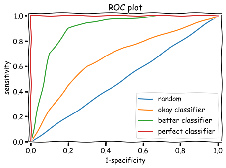
A nice way to visualize the tradeoff between sensitivity and specificity for different thresholds is a ROC plot (often pronounced 'rock plot'). ROC plots compare the performance of binary classifiers (i.e. a model that sorts inputs into positives and negatives). To generate a ROC curve, we plot FPR vs. TPR, or 1-specificity vs. sensitivity at each threshold.

By looking at this plot, you can see how true positives and false positives vary as you change the threshold. If you make the threshold very high, you need a very high log-odds score to be classified as positive (sleek) – you will probably have a very low false positive rate, but you will probably also have a very low true positive rate, losing a lot of the actual sleek songs. Alternatively, if you make the threshold very low, you will probably classify all of your positive (sleek) sequences as sleek, but you will also misclassify a lot of negative (fluffy) sequences as sleek.
You can use a ROC plot to determine what your threshold will be – for example, you may want a low false positive rate of 5% or less, and a ROC plot will help you find the corresponding score threshold to achieve this.
False discovery rate (FDR)
As mentioned in class, ROC plots can be deceiving when you have very high background – very few sleek sequences and very many fluffy sequences. At this point, even if you have high sensitivity, and identify a large fraction of the sleek sequences, you will also identify many fluffy sequences as belonging to sleek. In this case, a useful metric is the false discovery rate:
- false discovery rate (FDR) = \(\frac{\mathrm{FP}}{\mathrm{FP+TP}}\)
The FDR tells you how much the noise is drowning out the signal. We'll also come back to this idea of FDR in future weeks and explore it further.
Practice problems
To try implementing your own Markov model for this example, download and complete these practice problems: w05-section-problems.ipynb. You will need the supplementary files: sleek_data.txt and fluffy_data.txt. And here are the solutions: w05-section-solutions.ipynb.