week 07: maximizing your expectations

This week we see a compact example in biological sequence analysis of a powerful philosophy of inference that I learned from David MacKay:

Write down the joint probability of everything in your problem (i.e. all the random variables).
Specify your generative probability model for the probability of the observed data, conditional on whatever needs to be in the model.
Use Bayes' rule and probability algebra to write down the probability of what you want to infer given what you observe (the data) and what you can actually calculate (the likelihood).
Specify any prior assumptions you were just forced to state.
Turn the crank.

Sometimes "turning the crank" means simple algebra, when our modeling problem only consists of observed data and some unknown parameters we want to infer.

But sometimes we need to deal with integrating over complicated distributions, or over additional hidden random variables in our problem that aren't the target of our inference. There is an arsenal of standard methods that go by names like expectation-maximization, Gibbs sampling, Markov chain Monte Carlo (MCMC), and variational inference, which are all part of MacKay's "turning the crank", readily adapted to any specific modeling problem.

Expectation-maximization algorithms are the gateway drug to this arsenal of techniques. Motif identification - inferring a short sequence motif shared by a set of longer sequences - is a wonderfully simple example of E-M.

sequence motifs

In week 02 and 05, we've already talked about sequence motifs and how to represent them with probabilistic position-specific weight matrices (PWMs).

Many DNA-binding and RNA-binding proteins recognize specific sequences, but few are so precise that they only recognize one sequence. Restriction enzymes that cut DNA at specific sites are probably the best example of DNA-binding proteins that recognize just a single sequence, such as EcoRI cleaving almost only at GAATTC sequences. Some other proteins have binding specificities that can be well represented by a consensus sequence, such as GANTC for the restriction enzyme HinfI or GTYRAC for HincII. Most, though, have only probabilistic preferences.

There are comprehensive collections of known PWMs, including the JASPAR database for DNA-binding transcription factors and RBPDB for RNA-binding proteins.

These probabilistic preferences can often be well approximated by a PWM, a short ungapped position-specific profile that assigns a probability $p_k(a)$ to each residue $a$ at each position $k$ of the motif.

If many examples of the motif have already been identified and aligned, then PWM parameters are simply estimated from observed counts of residues in each position. For example, in week 02 we saw this example alignment:

seq1   GATTACA
seq2   GAATAGA
seq3   GAGTGTA
seq4   GACAAAA

which becomes a PWM of width W=7 with 4*7=28 probabilities:

A       0 1.0 0.25 0.25 0.75 0.25 1.0
C       0   0 0.25    0    0 0.25   0
G     1.0   0 0.25    0 0.25 0.25   0
T       0   0 0.25 0.75    0 0.25   0

There are many kinds of experiments that identify only the approximate location of a binding site. For example, we can fragment chromatin and use an antibody to pull down our favorite transcription factor, with whatever DNA fragments it is bound to, and sequence those fragments - a so-called chromatin immunoprecipitation and sequencing experiment, ChIP-seq. Now we have a set of longer DNA sequences (maybe 100-500nt long), each of which is likely to contain a short binding site motif, but we don't know where that motif is in each fragment.

If I told you the location of each motif, you would be able to pull them out of the longer fragments, make a multiple sequence alignment, and estimate a PWM. If I told you the PWM, you would be able to scan it across each fragment, and infer where the highest scoring (highest posterior probability) location. But if I give you just a set of N fragment sequences of length L, each of which contains a motif of length W, can you infer both the motif locations and the PWM?

This is where the expectation-maximization algorithm comes in.

bacterial ribosome binding sites

For this week's homework, our motif-finding example uses bacteriophage ribosome binding sites.

In a bacterial messenger RNA, the translational initiation site is recognized by the small subunit of the ribosome (SSU). The SSU, with a formylmethionine (fMet) initiator tRNA in its P site, binds by base-pairing to the fMet anticodon to the initiation codon, usually an AUG. The SSU simultaneously recognizes a short motif upstream of the AUG called a Shine/Dalgarno (S/D) sequence, by base-pairing to the 3' end of the SSU ribosomal RNA. The combination of the S/D, a short gap of maybe 4-10nt, and the AUG are called the ribosome binding site (RBS).

An E. coli S/D has a rough consensus of GGAGG, with a lot of variation. The 3' end of E. coli SSU rRNA is 5'-UCCUCCUUA-3'. Strong ribosome binding sites tend to have better complementarity to the SSU rRNA (up to 7-9 nucleotides: UAAGGAGGA is amongst the strongest). Weak ribosome binding sites for low-expressed proteins might only have 3-4 nucleotides of complementarity anywhere along the 3' end of SSU, such as AGGA, GGAG, or GAGG.

In our homework problem, we will model the S/D with a fixed-length PWM of some length W, choosing W in the range of maybe 4-8.

the generative probability model for motif inference

Following the MacKay philosophy, let's first establish our probability model, with our notation.

The observed sequence data $X$ consist of $N$ DNA sequences of length $L$. $X^s$ is sequence $s$, where $s=1 \ldots N$. $X^s_i$ is residue $i$ in sequence $s$, for $i=1 \ldots L$.

A PWM of width $W$ is $p_k(a)$, for positions $k=1 \ldots W$ and residues $a = A|C|G|T$.

Each observed sequence $X^s$ has exactly one motif in it, at position $\lambda^s$. $\lambda^s$ is $1 \ldots L-W+1$ (because there's an edge effect; to have a complete motif, it can't start at the rightmost edge of the sequence).

We assume that these motif positions are uniformly random a priori: $P(\lambda^s) = \frac{1}{L-W+1}$.

Outside of where the motif is, the rest of the observed sequence is modeled as i.i.d. background, with probabilities $f(a)$.

I'll refer to the combination of the PWM probabilities $p_k(a)$ and the background probabilities $f(a)$ as "the model", and sometimes represent all those probability parameters with $\theta$ as a typical shorthand for "all the model parameters". Note that we're going to estimate the background probabilities as part of the model. The observed sequences might have biased sequence composition, and we don't want to just find AT-rich motifs in AT-rich sequence.

This is a complete generative model of the observed sequences. We know the model is a complete generative model because we can see we have specified everything we need to generate a synthetic positive control dataset: we would choose a PWM of width $W$ and background frequencies $f$, and then generate $N$ sequences of length $L$ by embedding a sampled motif (sampled from $p$) in a background sequence (sampled from $f$) at random positions $\lambda$ (sampled uniformly).

If you knew the $\lambda^s$ positions, you would just extract the individual motifs from each sequence, align them (put them in register, in columns 1..W), and collect the observed counts of residues $c_k(a)$ for each motif position $k$ and each residue $a$. Given those counts, your maximum likelihood estimate for the PWM $p$ is just to use the residue frequencies at each position:

$$ p_k(a) = \frac{c_k(a)} {\sum_b c_k(b)} $$

Our problem is, the $\lambda^s$ are not known. The $\lambda$ motif positions are hidden variables: we do not directly observe them in the observed sequence data, but we need to know them to calculate the probability of the data. Hidden variables are common in probabilistic modeling, when there's some sort of hidden "state" of the data that we're not observing (like, is this residue $x_i$ in the motif or not, and if so at what position).

If you knew $\theta$, you could use probability algebra to obtain a posterior probability distribution for inferring the unknown motif position $\lambda^s$ in each sequence:

$$ P(\lambda^s \mid \theta, X^s) = \frac{P(X^s \mid \theta, \lambda^s) P(\lambda^s)} {\sum_{\lambda=1}^{L-W+1} P(X^s \mid \theta, \lambda) P(\lambda)} $$

The likelihood term in that is what we know how to put numbers to and calculate: In a real implementation, it's numerically safer to do this as a log likelihood, summing log terms instead of multiplying probabilities and risking underflow.

$$ P(X^s \mid \theta, \lambda^s) = \prod_{i=1}^{\lambda^s-1} f(X^s_i) \prod_{k=1}^{W} p_k(X^s_{\lambda^s+k-1}) \prod_{i=\lambda^s+W}^{L} f(X^s_i) $$

And we stated that a uniform prior for the $P(\lambda^s)$ term, $P(\lambda^s) = \frac{1}{L-W+1}$.

expectation-maximization

We have a chicken-and-egg problem. If we knew the motif positions $\lambda$, we could estimate a model $\theta$. If we knew the model $\theta$, we could infer motif positions $\lambda$. But we don't know either; we just have the observed long sequences $X$.

The key idea of E-M is to solve this chicken-and-egg problem iteratively. Given a current guess for $\theta$, infer $\lambda$ and use that to collect expected counts $c_k(a)$ and $c(a)$ for a new PWM and background frequencies (this is the expectation step). Then given expected counts $c_k(a)$ and $c(a)$, infer maximum likelihood parameters for the new PWM $p_k(a)$ and background probabilities $f(a)$ (the maximization step). Iterate these E-M steps until the model converges.

How do you initialize this iterative algorithm? Remarkably, E-M will typically work even starting from a random guess at either of the unknowns - either a random motif position $\lambda^s$ in each sequence, or random probability parameters in the PWM and background.

The expectation step comes in two pieces. First we calculate the posterior probability distribution $P(\lambda^s \mid \theta, X^s)$ for the unknown motif position in each sequence $X^s$. Then we collate expected counts by weighting every possible $\lambda^s$ position according to its posterior probability of being the motif start position:

$$ c_k(a) = \sum_{s=1}^N \sum_{\lambda^s=1}^{L-W+1} P(\lambda^s \mid X^s, \theta) \; \delta(X^s_{\lambda^s+k-1} = a) $$

A "Kronecker delta" is a notational convenience that takes the value 1 when its condition is true, else 0.

which may look harder than it really is, with that Kronecker delta in the notation, and those $s$ superscripts. In words:

for each sequence $X^s$:
calculate the posterior distribution $P(\lambda^s \mid X^s, \theta)$ as above;
for each possible motif position $\lambda^s = 1..L-W+1$ in the sequence:
- for each column $k$ of the PWM:
  - When you've got the PWM aligned at start position $\lambda^s$, residue $X^s_{\lambda^s+k-1}$ in the sequence is aligned to position $k$ in the PWM. Call this residue $a$.
  - Add a fraction of a count, $P(\lambda^s \mid x^s, \theta)$, to $c_i(a)$.

The background frequencies are updated in a similar way, just collecting weighted expected counts outside the motif, from positions $1 \ldots \lambda^s-1$ and $\lambda^s+W \ldots L$, again weighted by the posterior $P(\lambda^n \mid x^n, \theta)$.

So the complete E-M algorithm is:

Initialize a starting guess at the PWM and background $\theta$ to anything (even random)
Iterate:
(Expectation:) Infer expected counts $c_k(a)$ for the motif and $c(a)$ for the background, given current $\theta$.
(Maximization:) Calculate updated $\theta$ given $c_k(a)$ and $c(a)$ counts.
until converged.

inferring probability parameters from counts

Let's look at the maximization step in a little more detail.

We have expected counts $c_i$ for a multinomial distribution over $n$ outcomes, and we want to infer probability parameters $p_i$. (This is the general problem we have at W PWM positions $p_k$, and the background distribution $f$; all are multinomial distributions over n=4 nucleotides.)

The maximum likelihood solution is simply to take the frequencies:

$$ \hat{p_i} = \frac{c_i}{\sum_j c_j} $$

I can derive that by writing down the log probability of the observed counts $c$ given the parameters $p$, differentiating with respect to the $p_i$, setting to zero, and solving. (Along with a trick called Lagrange multipliers, for enforcing the constraint that $\sum_i p_i = 1$.)

When I have a lot of counts, I get a pretty accurate estimate of my $p_i$. But when I only have a few counts, my estimate will be noisy. Worse, I might observe 0 counts of some outcomes, and if I infer that these outcomes have zero probability, my parameterized model will inflexibly reject those outcomes as impossible. I may want to do something to avoid inferring any $p_i = 0$.

There is a common trick of adding a "pseudocount": This trick is sometimes called "Laplace's law of succession". Laplace was first to derive it formally.

$$ \hat{p_i} = \frac{c_i + 1}{\sum_j c_j + 1} $$

More generally, we might use a pseudocount $\alpha$ other than 1, or even a different $\alpha_i$ for every outcome:

$$ \hat{p_i} = \frac{c_i + \alpha_i}{\sum_j c_j + \alpha_j} $$

The higher the $\alpha_i$ pseudocounts, the more observed data it takes to override the pseudocounts.

Is there an optimal choice of $\alpha_i$? It turns out that these terms arise from a Bayesian view of the parameter inference problem, where we have a Dirichlet prior $P(\vec{p} \mid \vec{\alpha})$ over all the possible choices of probability vector $\vec{p}$, and we calculate a mean posterior estimate for $\vec{p}$. A uniform Dirichlet prior corresponds to Dirichlet prior parameters $\alpha_i = 1$. Different choices of $\alpha_i$ correspond to specifying different prior distributions over $\vec{p}$. We won't delve much into Dirichlets much, except for a bit more on them at the end of the notes today, on using a Dirichlet to sample random probability parameter vectors.

practicalities

relative entropy revisited

How do we think about the "consensus" of a PWM? We could simply just take the maximum probability residue at each position as the consensus. However, because we can have nonuniform background probabilities with a strong bias (AT-bias or GC-bias, in the pset this week), we may want to think in information theoretic terms, comparing the two distributions.

We can convert each PWM probability term to a log-likelihood ratio score (comparing to the background frequencies), and then calculate the average expected score of a motif:

$$ \sum_{k=1}^{W} \sum_{a=A}^{T} p_k(a) \log_2 \frac{p_k(a)}{f(a)} $$

we get the relative entropy score, a quantity in bits that also happens to be the Kullback-Leibler divergence between the PWM $p$ and the iid background $f$.

This is a good number to judge the "strength" of a motif by. A higher relative entropy means a PWM that is more distinct from the background.

If the background frequencies were uniform, this simplifies to 2W - H, where H is the entropy (in bits) of the PWM, $\sum_k \sum_a p_k(a) \log_2 p_k(a)$. This is often called the "information content" of a motif.

When people plot sequence logos, they typically calculate the information content per position, $I_k = 2 - \sum_a p_k(a) \log_2 p_k(a)$, and then plot each letter with a height of $p_k(a) \cdot I_k$.

Remember in these calculations that $\lim_{p \rightarrow 0} p \log p = 0$, so you avoid illegal $\log 0$ calls by treating any $p \log p$ term as 0 when $p=0$.

summing probabilities stored in log space: logsumexp

When calculating posterior probabilities, you have a denominator that is a sum over likelihood multiplied by prior. In an implementation, you're typically calculating log likelihoods and storing values as log probabilities. How do you sum in "probability space", when you're storing values in "log space"? You can't just exponentiate the log probabilities, sum, and take the log. The main reason you're storing numbers as log probabilities is to avoid underflow. If you exponentiate a log probability term, you may underflow.

There is a standard trick for this called the "logsumexp" trick. It goes like this.

Suppose I have probabilities $a$ and $b$ and I want to calculate $a+b = c$; but I am storing the probabilities as $A = \log a$ and $B = \log b$, and I want the answer to stay stably in log space too, $C = \log c$. How do I calculate $C = \log( a + b)$, given A and B?

$$ \begin{eqnarray} C & = & \log (e^A + e^B) \ & = & \log (e^A (1 + e^{B-A})) \ & = & A + \log(1 + e^{B-A}) \end{eqnarray} $$

$e^{B-A}$ might underflow, but now we don't care. If $e^{B-A}$ underflows, that means $B << A$ and $C \simeq A$.

The logsumexp trick generalizes to any number of terms. Suppose I want $Y = \log \sum_i x_i$, given $X_i = \log x_i$. Let $\hat{X} = \max_i X_i$ be the maximum of those terms. Then:

$$ Y = \hat{X} + \log \sum_i e^{X_i - \hat{X}} $$

where we note that $e^{\hat{X} - \hat{X}}$ = 1.

NumPy provides numpy.logaddexp() for the simple two-term version, and SciPy provides scipy.special.logsumexp() for the generalization to summing log probability vectors in probability space. Both work in natural log (nats). If your log probabilities are in base two (bits), you need to roll your own logsumexp2() routine.

local optima

Generally, EM is a local optimizer. For many problems that it is applied to, different initialization starting guesses will yield different optima, if the posterior probability surface for $P(\theta \mid \mathrm{data})$ is rough.

When dealing with a local optimizer, you want to re-run your algorithm at least a few times from different starting points, and choose the best result. "Best" is usually judged by the total log likelihood of the observed data given your model, $\log P(\mathrm{data} \mid \theta)$. Here, calculating the log likelihood for each observed sequence requires a marginal sum over the possible motif positions.

initialization strategies

A variety of initialization strategies work for EM algorithms for motif identification. Some options include:

Initialize with uniformly random motif positions $P(\lambda^s \mid \cdot)$; collect expected counts and estimate probabilities for $\theta$.
Initialize with a randomly chosen motif position in each sequence, sampled with uniform probability $\frac{1}{L-W+1}$, collect expected counts and estimate $\theta$.
Initialize the model $\theta$ with random probability parameters $p_k(a)$ and $f(a)$.

The first option is deterministic - it always gives you the same initialization point. That's undesirable from the standpoint of wanting to re-run a local optimizer from different starting points.

The third option requires knowing how to sample random probability parameters. We'll talk about that in a subsequent section.

convergence tests

How many iterations of EM should you do? You might get by with "a lot", if compute time is not limiting. For this week's pset, I started just by doing a fixed number of 50-100 iterations. But it's a little more sophisticated to have a convergence test of some sort.

You can look at how much the total log probability of the data improved from one iteration to the next, and set some fractional epsilon as your connvergence criterion. I've seen situations where the log likelihood is skating along some sort of plateau in the likelihood surface, but the model is actually changing quite a bit. So another convergence test is to look at how much the model changed from one iteration to the next, perhaps by calculating a Kullback-Leibler divergence.

There's no right answer. Different problems have different characteristics. I will typically start by doing an excessive number of iterations on synthetic positive control data where I know the right answer, and then develop a better convergence criterion to save wasting unnecessary compute.

sampling random probability vectors: the Dirichlet

Is there a way to sample a multinomial probability vector $\vec{p} = p_1 \ldots p_n$ uniformly, from all possible probability vectors?

This has us talking about sampling from a probability distribution over probability vectors, $P(\vec{p})$. We will need to think about such things, because in some Bayesian inference problems, we may want to specify an informative nonuniform prior over unknown model probability parameters. Thinking about how to sampling from a uniform $P(\vec{p})$ is one place to get started.

You might think you could just sample each individual $p_i$ uniformly on 0..1 (using Python's rng.random(), for example) -- i.e. $p_i == u_i$, for a uniform random variate $u_i = [0,1]$, but of course that doesn't work, because they're constrained to be probabilities that sum to one: $\sum_i p_i = 1$.

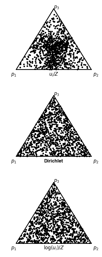
One bad way and two good ways to sample probability vectors uniformly. The examples show 1000 samples, plotted in so-called "barycentric" coordinates (also known as a "ternary plot"), to show the 3D simplex in 2D. The top panel (the bad way) shows sampling by drawing uniform variates and renormalizing. The middle panel shows sampling from a Dirichlet distribution with all alpha=1. The bottom panel shows sampling uniform variates, taking their log, and renormalizing.

So then you might think, ok fine, I'll sample elements uniformly then renormalize the vector: $p_i = \frac{u_i}{\sum_j u_j}$. Alas, this doesn't sample probability vectors uniformly, as shown by the clustering of samples in the middle of in the top panel of the figure to the right.

The right way to do it is to use the Dirichlet distribution. The Dirichlet is a distribution over multinomial probability vectors:

$$ P(\vec{p} \mid \vec{\alpha}) = \frac{\prod_{i=1}^{K} p_i^{\alpha_i-1} } {Z(\vec{\alpha})} $$

where the normalization factor $Z(\vec{\alpha})$ is:

$$ Z = \frac{\prod_i \Gamma(\alpha_i) }{\Gamma \left( \sum_i \alpha_i \right)} $$

With all $\alpha_i=1$, all probability vectors are sampled uniformly, because the $p_i^{\alpha_i-1}$ term becomes a constant $p_i^0 = 1$ for all values of $p_i$.

So if you go over to Python's np.random.dirichlet, you'll find that you can do:

   import numpy as np
   p = np.random.dirichlet(np.ones(n))

and you'll get a uniformly sampled probability vector $\vec{p}$ of size $n$. That's illustrated in the middle panel to the right.

Then it turns out that in the special case of all $\alpha_i = 1$, you can prove that sampling uniformly from the Dirichlet is equivalent to taking the logarithm of uniform variates and renormalizing,

$$ p_i = \frac{\log(u_i)} {\sum_i \log(u_i)} $$

This special case might be useful to know, like if you're programming in a language other than Python that doesn't put a np.random.dirichlet so conveniently at your fingertips. The bottom plot of the figure to the right shows using the $\log(u_i)/Z$ method.

If you want to play around with this, you can download the script I used to generate the figure.

The Dirichlet distribution will turn out to be useful to us for other reasons than just sampling uniformly-distributed probability vectors, as the next section delves further into.

digitizing sequences

You might find it useful to convert a DNA sequence as a string (e.g. "GATTACA") into an array of integer 0-3 indices representing each residue, A=0, C=1, etc. I use idioms like this to "digitize" input sequences:

    X = [ 'ACGT'.find(a) for a in seq ]

and now for seq = "GATTACA", X = [ 2, 0, 3, 3, 0, 1, 0], and I can use X[i] as an array index directly: for example in something like p[k][X[i]].

w00: intro	lecture	section	"pset"	"answers"
w01: genomes	lecture	[molbio] [py]	pset	answers
w02: probability	lecture	section	pset	answers
w03: data	lecture	section	pset	answers
w04: alignment	lecture	section	pset	answers
w05: Bayes	lecture	section	pset	answers
w06: p-values	lecture	section	pset	answers
w07: EM	lecture	section	pset	answers
w08: HMMs	lecture	section	pset	answers
w09: k-means	lecture	section	pset	answers
w10: regression	lecture	section	pset	answers
w11: PCA	lecture	section	pset	answers
w12: work	lecture	-	-	-
w13: trees	lecture	section	pset	answers