week 02: and now for some probability
Probability theory is nothing more than common sense reduced to calculation.
- Pierre-Simon Laplace (1819).
the probability of boys and girls
In the 1770's, the French mathematician Pierre Laplace started working on big data.
Laplace became interested in the curious biological observation that the ratio of boys to girls at birth isn't exactly 50:50. Village records showed an apparent bias towards more boy births, but the numbers were small and vulnerable to statistical fluctuation. Laplace set out to use some new ideas he had about probability theory to put the question of sex ratio at birth to a mathematically rigorous test, and he needed big data sets to do it. "It is necessary to make use in this delicate research much greater numbers", Laplace wrote in his classic 1781 paper.
Laplace turned to the extensive census records in London and Paris. The Paris census for the years 1745-1770 recorded the birth of 251527 boys and 241945 girls, a 51:49 (1.04) ratio. The London census for 1664-1757 recorded the birth of 737629 boys and 698958 girls, again a 51:49 ratio.
Laplace's work is one of the origins of probability theory. Today, his laborious manual calculations are easy to reproduce in a few lines of Python. His problem makes a compact, biologically-motivated example for us to illustrate some of the key ideas of probabilities and probabilistic inference. The bias in the human male/female ratio at birth is real and it remains poorly understood. It is typically measured at 1.02 to 1.08 in different human populations.
the binomial distribution
Let's call the probability of having a boy \(p\). The probability of having a girl is \(1-p\). The probability of having \(b\) boys in \(N\) total births is given by a binomial distribution:
A couple of things to explain, in case you haven't seen them before:
-
\(P(b \mid p,N)\) is "the probability of b, given p and N": a conditional probability. The vertical line \(\mid\) means "given". That is: if I told you p and N, what's the probability of observing data b?
-
\({ N \choose b }\) is conventional shorthand for the binomial coefficient: \(\frac{N!}{b! (N-b)!}\).
Suppose \(p=0.5\), and \(N=493472\) in the Paris data (251527 boys + 241945 girls). The probability of getting 251527 boys is:
Your calculator isn't likely to be able to deal with that, but Python
can. For example, you can use the pmf (probability mass function) of
scipy.stats.binom:
    import scipy.stats as stats
    p = 0.5
    b = 251527
    N = 493472
    Prob = stats.binom.pmf(b, N, p)
    print(Prob)
which gives \(4.5 \cdot 10^{-44}\).
Probabilities sum to one, so \(\sum_{b=0}^{N} P(b \mid p, N) = 1\). You can verify this in Python easily, because there are only \(N+1\) possible values for \(b\), from \(0\) to \(N\).
maximum likelihood estimate of p
Laplace's goal isn't to calculate the probability of the observed data, it's to infer what \(p\) is, given the observed census data. One way to approach this is to ask, what is the best \(p\) that explains the data -- what is the value of \(p\) that maximizes \(P(b \mid p, N)\)?
It's easily shown In this case, "it's easily shown" means we take the derivative of \(P(b \mid p, N)\) with respect to \(p\), set to zero, and solve for \(p\). Also, if we're being careful, then we take the second derivative at that point and show that it's negative, so we know our extremum is a maximum, not a minimum. Typically -- though it turns out not to be necessary in this particularly simple case -- you would also impose constraint(s) that probability parameters have to sum to one, using the constrained optimization technique of Lagrange multipliers. See, that stuff you learned in calculus is useful. that this optimal \(p\) is just the frequency of boys, \(\hat{p} = \frac{251527}{493472} = 0.51\). The hat on \(\hat{p}\) denotes an estimated parameter that's been fitted to data.
With \(\hat{p} = 0.51\), we get \(P(b \mid \hat{p}, N) = 0.001\). So even with the best \(\hat{p}\), it appears to be improbable that we would have observed exactly \(b\) boys. But that's simply because there's many other \(b\) that could have happened. The probability of the data is not the probability of \(p\); \(P(b \mid p,N)\) is not \(P(p \mid b, N)\). When I deal you a draw poker hand, it's laughably unlikely that I would have dealt you exactly those five cards in a fair deal, but that doesn't mean you should reach for your revolver.
It seems like there ought to be some relationship, though. Our optimal \(\hat{p}=0.51\) does seem like a much better explanation of the observed data \(b\) than \(p=0.5\) is.
\(P(b \mid p, N)\) is called the likelihood of \(p\), signifying our intuition that \(P(b \mid p,N)\) seems like it should be a relative measure of how well a given \(p\) explains our observed data \(b\). We call \(\hat{p}\) the maximum likelihood estimate of \(p\).
The London and Paris data have different maximum likelihood values of \(p\): 0.5135 versus 0.5097. Besides asking whether the birth sex ratio is 50:50, we might even ask, is the ratio the same in London as it is in Paris?
the probability of p
Laplace made an intuitive leap. He reasoned that one value \(p_1\) is more probable than another \(p_2\) by the ratio of their likelihoods:
if we had no other reason to favor one value for \(p\) over the other. We'll see later that this means that Laplace implicitly assumed a uniform prior for \(p\).
So \(p=0.51\) is \(\frac{0.001}{4.5e-44} \sim 10^{40}\)-fold more probable than \(p=0.5\), given the Paris data.
This proportionality implies that now we can obtain a probability distribution for \(p\) by normalizing over the sum over all possible \(p\) -- which requires an integral, not just a simple sum, since \(p\) is continuous:
This is a probability density, because \(p\) is continuous. Strictly speaking, the probability of any specific value of \(p\) is zero, because there are an infinite number of values of \(p\), and \(\int_0^1 P(p \mid b, N) \: dp\) has to be 1.
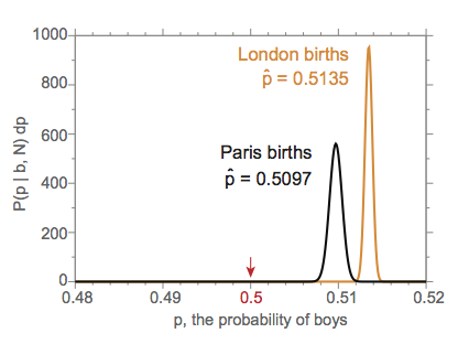
It's possible (and indeed, it frequently happens) that a probability density function like \(P(p \mid b, N)\) can be greater than 1.0 over a small range of \(p\), so don't be confused if you see that; it's the integral \(\int_0^1 P(p \mid b, N) \: dp = 1\) that counts. For example, you can see that there are large values of \(P(p \mid b, N) \: dp\) in the figure above, where I've plotted Laplace's probability densities for the Paris and London data.
In the figure, it seems clear that \(p = 0.5\) is not supported by either the Paris or London data. We also see that the uncertainty around \(p^{\mathrm{london}}\) does not overlap with the uncertainty around \(p^{\mathrm{paris}}\). It appears that the birth sex ratio in Paris and London is different.
We're just eyeballing though, when we say that it seems that the two distributions for \(p\) don't overlap 0.5, nor do they overlap each other. Can we be more quantitative?
the cumulative probability of p
Because the probability at any given continuous value of \(p\) is actually zero, it's hard to frame a question like "is \(p = 0.5\)?". Instead, Laplace now framed a question with a probability he could calculate: what is the probability that p <= 0.5?, If that probability is tiny, then we have strong evidence that \(p > 0.5\).
In the homework this week, we'll see the complementary cumulative probability distribution, also known as a survival function, which is \(P(X>x)\). This appears a lot in biological sequence analysis when X is a score -- maybe a sequence alignment score, from some sort of database search -- and we're interested in the probability that we get a score above some threshold \(x\) in a negative control experiment (null hypothesis) of some sort, because we want to set a threshold for a statistically significant result.
A cumulative probability distribution \(F(x)\) is the probability that a variable \(X\) takes on a value less than or equal to \(x\), \(P(X \leq x)\). For a continuous real-valued variable \(x\) with a probability density function \(P(x)\), \(F(x) = \int_{-\infty}^x P(x)\). For a continuous probability \(p\) constrained to the range \(0..1\), \(F(p) = \int_0^p P(p)\) and \(p \leq 1\).
So Laplace framed his question as:
Then Laplace spent a bazillion pages working out those integrals by hand, obtaining an estimated log probability of -42.0615089 Yes, Laplace gave his answer to 9 significant digits. Showoff. (i.e. a probability of \(8.7 \cdot 10^{-43}\)): decisive evidence that the probability \(p\) of having a boy must be greater than 0.5.
These days we can replace Laplace's virtuosity with one Python call:
   import scipy.special as special
   p = 0.5
   b = 251527
   N = 493472

   answer = special.betainc(b+1, N-b+1, p)
   print (answer)
which gives \(1.1 \cdot 10^{-42}\). Laplace got it pretty close -- though it was quite a waste of sig figs.
Beta integrals
Wait, what sorcery is this betainc() function?
That
betainc
call is something called a Beta integral. Let's take a little
detour-dive into this.
The complete Beta integral \(B(a,b)\) is:
A gamma function \(\Gamma(x)\) is a generalization of the factorial from integers to real numbers. For integer \(a\),
and conversely
The incomplete Beta integral \(B(x; a,b)\) is:
and has no clean analytical expression, but statistics packages
typically give you a computational method for calculating it -- hence
the SciPy scipy.special.betainc
call.
If you wrote out Laplace's problem in terms of binomial probability distributions for \(P(b \mid p, N)\), you'd see the binomial coefficient cancel out (it's a constant with respect to \(p\)), leaving:
Alas, reading documentation in Python is usually essential, and it
turns out that the
scipy.special.betainc
function doesn't just calculate the incomplete beta function; it
sneakily calculates a regularized incomplete beta integral
\(\frac{B(x;a,b)}{B(a,b)}\) by default, which is why all we needed to
do was call:
answer = special.betainc(b+1, N-b+1, p)
Beta integrals arise frequently in probabilistic inference. When we extend them beyond just \(K=2\), we can deal with data from dice and DNA and proteins (\(K=6,4,20\)), generalizing the binomial distribution to the multinomial distribution, and the Beta integral to the multivariate Beta integral.
summary
Laplace treated the unknown parameter \(p\) like it was something he could infer, and express an uncertain probability distribution over it. He obtained that distribution by inverse probability: by using \(P(b | p)\), the probability of the data if the parameter were known and given, to calculate \(P(p | b)\), the probability of the unknown parameter given the data.
Laplace's reasoning was clear, and proved to be influential. Soon he realized that the Reverend Thomas Bayes, in England, had derived a very similar approach to inverse probability just a few years earlier. We'll learn about Bayes' 1763 paper later in the course. But for now, let's leave Laplace and Bayes, and lay out some common-sense usage of probabilities in sequence analysis.
the probability of a sequence
For many common sequence analysis problems, we want to be able to express the probability of a sequence \(x_1..x_L\) of length \(L\). Let's make it a DNA sequence, with an alphabet of 4 nucleotides ACGT, to be specific; but it could also be a protein sequence with an alphabet of 20 amino acids, or indeed some other kind of symbol string.
We'll see more on the justification for log-likelihood ratio scores below. Why would we want to express the probability of a sequence, you ask? One good starting example is, suppose there are two different kinds of sequences with different statistical properties, and we want to be able to classify a new sequence (a binary classification problem). We want to express \(P(\mathbf{x} \mid H_1)\) and \(P(\mathbf{x} \mid H_2)\) for two probability models of the two kinds of sequences. Using those likelihoods, we can calculate a score - a log likelihood ratio, \(\log \frac{P(\mathbf{x} \mid H_1)}{P(\mathbf{x} \mid H_2)}\), as a well-justified measure of the evidence for the sequence matching model 1 compared to 2.
For interesting sequence lengths \(L\), we aren't going to be able to express \(P(x_1..x_L \mid H)\) directly, because we'd need too many parameters: \(4^L\) of them, for DNA. We need to make assumptions: we need to make independence assumptions that let us factorize the joint probability \(P(x_1..x_L \mid H)\) in terms of a smaller number of parameters.
the i.i.d. sequence model
For example, we could simply assume that each nucleotide \(a\) is drawn from a probability distribution \(p(a)\) over the four nucleotides, and each nucleotide \(x_i\) in the sequence is independently drawn from the identical distribution. Then:
This is about the simplest model you can imagine. It is called an independent, identically distributed sequence model, or just i.i.d. for short. If someone says an "i.i.d. sequence", this is what they mean. We use independence to factor the probability \(P(x_1..x_L)\) into a product of probabilities for each symbol. We additionally assume that the distribution of symbol probabilities \(p(x)\) is identical at every position.
You could make two i.i.d. models \(H_1\) and \(H_2\) with different base composition -- one with high probabilities for AT-rich sequence, the other with high probabilities for GC-rich sequence -- and you'd have the basis for doing a probabilistic binary classification of sequences based on their nucleotide composition.
position-specific scoring models for motifs
Suppose you have a multiple sequence alignment (MSA) of a conserved sequence motif:
seq1   GATTACA
seq2   GAATAGA
seq3   GAGTGTA
seq4   GACAAAA
This example has a consensus GANWRNA. (The R stands for purine A|G, W for "weak" A|T, and N for any residue A|C|G|T.) If we want to identify more examples of this conserved motif in genome sequences, we could use a pattern-matching algorithm (a regular expression) to look for sequences that match that consensus. But a consensus pattern match lacks subtlety - it either matches or it doesn't. It's not capable of distinguishing quantitatively between degrees of evolutionary conservation. Shouldn't a position that's 99% A give a higher score to matching an A than a position that's only 80% A? For instance, for that W at consensus position 5, it's more T than A there; shouldn't T get a higher score?
So it's easy to imagine that what we want is some sort of position-specific scoring matrix (PSSM), also more commonly known as a position-specific weight matrix (PWM), that captures the primary sequence consensus in a more quantitative way. For each position (consensus column) of the MSA, we want to assign a score for A|C|G|T, such that probable symbols have good scores and improbable symbols have bad scores. For a putative target sequence \(x_1..x_L\), we would add up the scores for each of its residues \(x_i\) according to the PWM.
Where should these scores come from? We get them from a probability model. I'll again defer a discussion of why we do it this way until later in the course, but here's what's done.
First we collect the observed counts at each position:
A     0 4 1 1 3 1 4
C     0 0 1 0 0 1 0
G     4 0 1 0 1 1 0
T     0 0 1 3 0 1 0
and then we use these counts to infer probabilities at each position, perhaps using the maximum likelihood estimate of simplying normalizing counts to frequencies:
A       0 1.0 0.25 0.25 0.75 0.25 1.0
C       0   0 0.25    0    0 0.25   0
G     1.0   0 0.25    0 0.25 0.25   0
T       0   0 0.25 0.75    0 0.25   0
Now we have a probability model for \(P(x_1..x_L)\) that says \(P(x_1..x_L) \simeq \prod_{i=1}^{L} p_i(x_i)\). Where the i.i.d. model assumed a single distribution \(p(x)\) for the symbol at any position \(i\), now we have L different probability distributions \(p_i(x)\), one for each position. We have \(4L\) parameters in our model, which is more than the 4 in the i.i.d. model, but far better than the \(4^L\) we would need to explicitly enumerate and parameterize \(P(x_1..x_L)\). To get that convenient collapse in how many parameters we need, we're still making the independence assumption, that each position is statistically independent of the others: this is a common assumption for primary sequence conservation models, including sequence alignment methods like BLAST.
We can sample from this distribution, perhaps to synthesize positive control data that matches what we expect our motif to look like, just by sampling each position according to these \(p_i(x)\) parameters.
Those zero probabilities might bother you, and they should. Is position 1 really always G? We only observed four sequences in our MSA. Shouldn't we allow for the possibility that our observed counts are just a statistical sample, and the frequencies are not the true probability parameters? Indeed we should - but again, I'll defer this out to later in the course, when we get a bit more machinery.
This is a probability model, but it's not the score model that we said we wanted -- it's not a PWM yet. We don't have scores we can add up for each position, we have probabilities that we multiply together. How do we get meaningful "scores"? Let's sneak up on that by taking a bit of a detour through a couple of other important concepts we need for manipulating probability models.
log likelihoods
Probabilities can get absurdly small pretty quickly, as you multiply together a bunch of probability parameters that are all between 0 and 1. Assuming uniform residue probabilities of 0.25 and a DNA sequence length of L=100, an i.i.d. DNA sequence probability \(P(x_1..x_L)\) is \(4^{-100} = 6e-61\).
This isn't only an inconvenience with working on pen and paper. It can be devastating in a computer because of numerical underflow. Python's double-precision floating point representation can only represent numbers down to about \(2.2e^{-308}\). Below that, the number just becomes 0 (the representation underflows). And this isn't the only gotcha in working with floating point numbers. If you try to add two numbers together, floating point math can only deal with the addition if they're relatively close to each other. There is a number \(\epsilon\) below which \(1 + \epsilon = 1\). In double-precision floating point, \(\epsilon\) is only about \(2.2e-16\). If you add (1 + 1e-20) the computer will get 1.
These problems are solved by working in "log space": working with log probabilities instead of probabilities. Where probabilities multiply, log probabilities sum. The log likelihood of our position-specific model is:
I could have used any base for the logarithm there. It would be more textbook-y to just leave it as the natural log, not \(\log_2\). But it turns out that we may as well get used to working in \(\log_2\) units, or "bits". Sequence analysis has a strong conceptual foundation in information theory and Shannon entropy, which historically use \(\log_2\) and bits ... as you know from working with computers, which also measure things in bits.
What do you do with \(\log_2 0\)? It's mathematically undefined, and
Python will rightly screech about it. In code, we have to explicitly
check that a probability \(p\) is \(> 0\) before we try to take a log, and
do something appropriate if it's 0. Sometimes the appropriate thing is
to treat \(\log_2 0\) as \(-\infty\). In Python, you'd do logp =
float('-inf').
Log likelihoods are \(\leq 0\). The highest/best log likelihood is 0, corresponding to a likelihood of 1. You sort of want a good score to be positive and a bad score to be negative, intuitively, so log likelihoods are a little weird to think about. Don't worry, we're about to fix that.
log-likelihood ratio scores
Continuing our conceptual detour, which will eventually bend back to a PWM:
A common sequence analysis problem is classification: we have probability models \(H_1..H_m\) for \(m\) classes, and we want to figure out how to classify a sequence \(x\). We'll see later in the course how Bayesian inference tells us to deal with a classification problem.
For now, suppose we're only talking about binary classification. I have two models \(H_1\) and \(H_2\). Then it turns out that a good score to calculate is the log-odds score, also known as a log likelihood ratio (LLR):
The LLR is positive if \(H_1\) fits the data better, negative if \(H_2\) is better, and zero if the two models explain the data equally well.
For example, \(H_1\) could be my position-specific probability matrix model and \(H_2\) could be an i.i.d. model. I could be trying to classify an input sequence as being a good match to the position-specific model, as opposed to a random null model of what background sequences look like.
I can algebraically rearrange the terms of the position-specific probability matrix and the i.i.d. model to express the LLR score for an input sequence as a sum of independent scores for each residue:
where here I used \(q(x)\) to represent the i.i.d. model parameters, to distinguish better from the position-specific \(p_i(x)\) parameters.
Thus I can take my probability matrix and precalculate a position-specific weight matrix by dividing each probability by its corresponding i.i.d. parameter (0.25 for uniform DNA) and taking the log2:
A       * +2  0    0  +1.6 0 +2
C       *  *  0    *    *  0  0
G      +2  *  0    *    0  0  0
T       *  *  0  +1.6   *  0  0
I used * characters there to represent -infinity's. This little example didn't happen to give me any negative scores, just because I didn't have any frequencies/probabilities less than 0.25.
It took a surprisingly long time for the computational biology field to arrive at this (correct) derivation for PWMs. PWMs are a good model for ungapped conserved sequences (no insertion and deletion) where we're willing to assume a model of primary sequence conservation alone. It took even longer for computational biology to arrive at a conserved consensus probability model that allows for gaps (profile hidden Markov models).
entropy and information
How conserved is each consensus column of a multiple sequence alignment? From the probability distribution \(p_i(a)\) for residues \(a\) at position \(i\), is there a good single number that represents how conserved that position is?
Shannon entropy
Claude Shannon
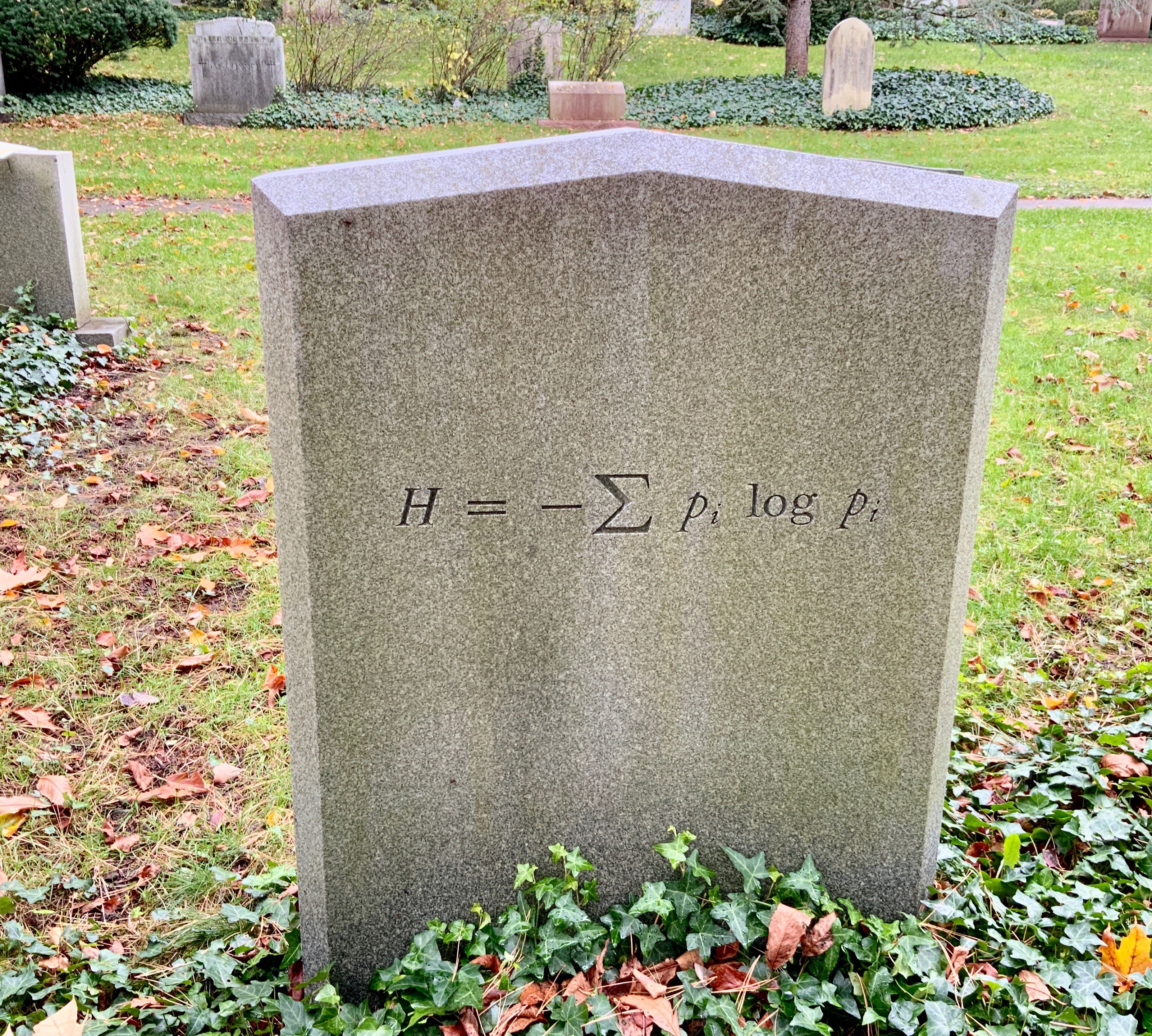 You can visit Claude Shannon's grave and pay your respects. He's
buried in Mount Auburn Cemetery right here in Cambridge. It's easy to
recognize, it's the gravestone with the entropy equation on it.
developed "information theory" and what we now call Shannon informational entropy.
You can visit Claude Shannon's grave and pay your respects. He's
buried in Mount Auburn Cemetery right here in Cambridge. It's easy to
recognize, it's the gravestone with the entropy equation on it.
developed "information theory" and what we now call Shannon informational entropy.
Shannon entropy starts from the idea that if the probability of an event \(x\) is \(p(x)\), then we can express our "surprise" at that outcome as \(\log_2 \frac{1}{p}\). A rare event of lower probability \(p(x)\) is more surprising than a common event, and Shannon intuited that a measure of "surprise" should be additive for independent events, hence the logarithm.
The intuition is easiest to see if we start with a uniform distribution over a number of events that's a power of 2. Suppose we're talking about the probability of four events A|C|G|T, the identity of a DNA nucleotide, with uniform probabilities \(p(x) = \frac{1}{4}\). The "Shannon information" of any of the 4 outcomes is 2 bits: \(\log_2 \frac{1}{0.25}\). If you had to ask binary yes/no questions to guess what nucleotide I was holding behind my back, it would take you 2 yes/no questions: "is it a purine"? yes. "is it a G"?
This intuition then extends to distributions over sample spaces that aren't a power of two in size. A fair die has six outcomes, with probabilities \(\frac{1}{6}\). If I roll a die and ask you to guess the outcome, it will take you \(\log_2 6 = 2.585\) yes/no questions on average to guess... if you have an optimal strategy for asking questions, over a large number of trials.
The intuition also extends to nonuniform distributions. If we have DNA residues and the probability of an A is 0.01, then the "surprise" of seeing A is high: \(\log_2 \frac{1}{0.01}\) = 6.64 bits, as if the event actually came from a uniform distribution over an effective number of \(\frac{1}{p(x)}\) = 100 outcomes.
Shannon's "source coding theorem" is too much to go into here, but it had a powerful take home message for data compression and communications theory: the optimal encoding of a symbol x in a binary code has length \(\log_2 \frac{1}{p(x)}\) bits.
It then makes sense to want to know the average encoding length required per symbol:
This is the famous equation for Shannon entropy. It's maximal for a uniform distribution (1 bit for a fair coin; 2 bits for uniform DNA nucleotides), and 0 if one of the probabilities is p(x)=1.
It measures how uncertain we are about the symbol: how many yes/no binary questions we would have to ask, on average, to obtain certainty.
The equation is usually shown as \(H(x) = - \sum_x p(x) \log_2 p(x)\) (even on Shannon's grave) but that obscures the intuition that the \(\log_2 \frac{1}{p(x)}\) term is the log of an effective number of outcomes.
The entropy of a multiple sequence alignment column is a good measure of conservation, with low entropy meaning high conservation.
Relative entropy; Kullback-Leibler divergence
We can compare two different probability distributions for the same set of outcomes with:
which measures the expected gain in information (in bits) from encoding symbols using distribution \(p\) (often the true distribution) versus distribution \(q\) (often the implied distribution for some binary encoding).
Since we just introduced log-likelihood ratio scoring: we also recognize this as an average LLR over data outcomes \(x\), for true distribution \(p\) and a null background distribution \(q\).
This quantity is often referred to as a Kullback-Leibler divergence. Sometimes people call it a "distance" but it's not a distance; it's not symmetric, \(\mathrm{KL}(p||q) \neq \mathrm{KL}(q||p)\) in general.
Mutual information
We can also compare a joint probability distribution of two outcomes to the product of their independent distributions. Suppose we have event \(i\) which results in an outcome \(a\), and a second event \(j\) with outcome \(b\). For example, we could be talking about what nucleotide A|C|G|T is in column \(i\) of a sequence alignment, and what is in column \(j\). We can calculate a mutual information:
The intuition for this value is, how much information (in bits) would I gain about the outcome at \(j\), if you tell me the outcome at \(i\) (and vice versa)?
The mutual information calculation is identical to the form of the Kullback-Leibler divergence: it's also the average information (in bits) that we gain by encoding the pair of events with a joint distribution, as opposed to the produce of their independent distributions.
Mutual information is a commonly used way of measuring pairwise correlation between columns of a multiple sequence alignment.
For example, in multiple alignments of homologous and conserved RNA structures, two positions in a consensus base pair may vary individually, while covarying to maintain the pair: an A paired to a U in one sequence might become a G paired to a C in a homolog. Conserved base pairs induce strong pairwise correlations in multiple sequence alignments because of these compensatory base pair substitutions over evolutionary time. Given a deep enough sequence alignment with enough variation, a simple mutual information calculation reveals the conserved structure by detecting these pairwise correlations. As we'll see in the pset this week!
the human genome is a 32-bit operating system
Shannon entropy gives us some powerful back-of-the-envelope intuition, Fermi estimation style, for sequence analysis.
The human genome contains about 3e9 bases, so if I'm trying to specify one location on the human genome, I need \(\log_2 3\mathrm{e}9 \simeq\) 32 bits of information to specify it. If I look for an exact ungapped match to a DNA motif of length W, that pattern has 2W bits of information in it (assuming a uniform distribution over DNA residues; human is actually 40% GC, but this is Fermi estimation). Therefore I know as a rule of thumb that I need around 16 nucleotides of exact match to specify one unique location in the human genome. (Ignoring repeats - again, Fermi style.)
If I search with a shorter pattern, I can quickly estimate how many hits I expect by chance alone. Say I search with a six-mer GAATTC (a restriction site for the EcoRI restricton endonuclease). That's a 2x6 = 12 bit pattern. 32 bits of positional uncertainty in the human genome minus a search with a 12 bit pattern = 20 bits of remaining uncertainty; I expect \(2^{20}\) = about a million hits to that pattern.
I can extend this intuition to ambiguity codes: if I search with the pattern GANWRNA, that's a 2 + 2 + 0 + 1 + 1 + 0 + 2 = 8 bit pattern.
I can also extend it to full probability models: I can use a relative entropy calculation to estimate the "information content" of any model relative to null background expectation, and use that to ballpark what my signal/noise is expected to be, in a database of any size. The current protein sequence databases are around 1 trillion amino acids big now. That's about 40 bits of uncertainty, so to find unique homologs well, I know I need search models or patterns with at least 40 bits of information in them.
practicalities this week
This week we introduce NumPy and Matplotlib for real. You might want to refer back to the w00 example pset, where I also showed examples of using them.
numpy arrays
Have a look at the Quick Start guide to NumPy, and its Absolute Basics for Beginners.
A numpy array stores a matrix of values all of the same type. It defaults to floats, but can also store integers or characters (and probably more but that's what I use it for). I use it for 1D vectors and 2D matrices most often, but it is also excellent at higher-dimensional tensors. That said, NumPy itself refers to all these things as "arrays" and explicitly prefers to avoid the mathematical terms vector, matrix, and tensor.
My cheat sheet includes things like:
Creating a new array, getting its size and stuff:
import numpy as np

A = np.array([0,1,2])              # np.array() converts anything list-like or N-dim array like to an ndarray
A = np.array([ [0,1,2], [3,4,5]])  #  ... here's a 2D example, from a list of lists
A = np.arange(12).reshape(3,4)     # np.arange() returns like range() but in an array of specified shape; .reshape() reshapes to a new shape (here, 3x4 from 12)

(nrows, ncols) = A.shape           # (3,4) : returns the "shape" of an array as a tuple
ndim = A.ndim                      # 2     : returns the dimensionality of an array
t    = A.dtype                     # dtype('int64') : returns the type of the array's values

p =  np.array([ [ 1/6, 1/6, 1/6, 1/6, 1/6, 1/6 ],      # probability distributions for a fair die and a loaded one
                [ 0.1, 0.1, 0.1, 0.1, 0.1, 0.5 ] ])
Other ways to create an array:
A = np.zeros(3)                 # [0.0,0.0,0.0]
A = np.zeros((2,3))             # 2x3 matrix.  shape is a tuple.
A = np.zeros(3).astype(int)     # integers [0,0,0].  The .astype() method converts dtype of the array.

A = np.ones((2,3))              # 2x3 matrix of 1's
A = np.empty((2,3))             #   ... or of uninitialized numbers

A = np.linspace(2, 100, 50)     # vector of 50 evenly-spaced numbers on closed interval [2,100]
Math with numpy arrays typically acts elementwise, so you can write many things compactly.
A = np.array([1,2,3])
B = A + A                  # [2,4,6].  You can add two arrays elementwise if they have the same shape.
C = A * A                  # [1,4,9].  Multiplication is elementwise. This is a reason that numpy doesn't call arrays "matrices": don't expect matrix multiplication
C = 1 + A                  # [2,3,4].  You can add a scalar to an array elementwise.
C = 0.5 * A                # [0.5,1.0,1.5]  ... or multiply elementwise, etc.
2D arrays are indexed (row, column), starting from 0. Shapes are expressed as tuples (nrows, ncolumns).
x = A[1,2]                 # you can ask for row 1, col 2 with a comma version
x = A[1][2]                # equivalent way to index: A[1] gives you row 1, and the [2] gives you element 2 from that
You can take subsets of an array by "slicing" operations.
A[:, [2,5]]    # select columns 2,5
A[:, 1:5]      # select columns 1..4
NumPy provides other functions - we've already seen random number generation. Here's some other useful ones:
log2p  = np.log2(p)     # base 2 log (works elementwise on arrays)
logp   = np.log(p)      # natural log
log10p = np.log10(p)    # base 10 log

denom  = np.sum(p)      # sum all the elements in an array - returns scalar
plotting with matplotlib
Matplotlib has an extensive user's guide including a quick start guide. But here are some basics, taken from my own work patterns and notes.
Imports (note the .pyplot submodule here:)
import matplotlib.pyplot as plt
import numpy as np
Matplotlib will let you use plt.* functions to make a single figure
(and you'll see Stack Overflow answers to this, etc.) but don't do it
that way. I find it better to use Matplotlib's object-oriented style
of creating and manipulating "Figure" and "Axes" objects:
fig, ax = plt.subplots() # default is 1 panel
A step more advanced, you can make multipanel figures:
fig, axs        = plt.subplots(2,2)                 # panel array, r x c: axs[0][0] or axs[0,0] etc
fig, (ax1, ax2) = plt.subplots(1,2)                 # can unpack array of panels into tuple(s)
fig, ((ax1, ax2), (ax3,ax4)) = plt.subplots(2,2)    # here, for a 2x2 grid
    figsize=(12,4)  # set figure size (x,y) in inches
    sharey=True     # y-axes use same scale (ticks).
    sharex=True     # x-axes, ditto
    layout=tight    # or: fig.tight_layout()
Each "Axes" object (here called ax) is one graph. You create it with
some sort of plotting function that you pass data to. Here's code to make
an example line, then plot it:
fig, ax = plt.subplots()

x = np.random.uniform(0, 100, 20)               # Sample 20 values  0 <= x < 100
y = np.add(np.multiply(x, 3.0), 5.0)            # y = mx + b  with slope 3.0, intercept 5.0
y = np.add(y, np.random.normal(0, 10.0, 20))    #    + N(0,10) noise

ax.plot(x,y)
You can add more lines to the same graph just by calling ax.plot()
for the data for each line you want to plot.
There's a whole bunch of customization for any plotting function, that you provide as keyword arguments. I consult its documentation, then play. For a line plot, some useful things:
ax.plot(x,y,
        color='orange',           # set line color. You can also use RGB hex codes e.g. '#ED820E'
        linestyle='--',           # '-' solid, '--' dashed, other choices exist
        linewidth=2,              # line width
        marker='o',               # '.' point, 'o' circle, 's' square; other choices exist
        markersize=6,             # sets data point marker size
        markerfacecolor='white',  # what color marker is filled with
        markeredgewidth='1.5')    # how big its edge is
Besides .plot(), there are many other functions for different types of
plots. Some important ones for us:
ax.scatter(x,y)         # plot x,y points as a scatter plot
ax.imshow(A)            # plot a numpy 2D array as a 2D grid: like for a heat map, for example
ax.hist(x)              # given a big list of numbers, bin them into appropriate bins and plot a histogram (as a bar graph)
ax.ecdf(x)              # given a big list of numbers, sort them and calculate/plot an empirical cumulative distribution function
Having plotted your data, you should then label your axes (of course), label your graph, and adjust other things to your liking:
ax.set_title('Title')
ax.set_xlabel('x axis label', c='gray', size=10)
ax.set_ylabel('y axis label', c='gray', size=10)
ax.legend() # toggle the addition of a legend

ax.set_xlim([20, 180])    # Set range of the x-axis
ax.set_ylim([0, 0.03])    #   ... and y axis
ax.set_yticks([-1.5, 0, 1.5])                                       # np.linspace(a,b,num=n)   [a,b] closed interval, n evenly spaced values.
ax.set_xticks(np.arange(0, 100, 30), ['zero', '30', 'sixty', '90']) # np.arange(a,b,s)         [a,b) half-open interval, step size of s. Best for

ax.tick_params(axis='both', which='major', direction='out', length=4, width=1.5, color='gray', labelcolor='gray', labelsize=8, labelfontfamily='Open Sans')
  # axis = 'both', 'x', 'y'
  # which = 'major', 'minor'
  # direction = 'out', 'in', 'inout'

ax.axis('equal')    # Make squares square
ax.set_axis_off()   # Turn off everything to do with both x and y axis: ticks, spines, labels. I used this for pset0 to just make a display scatterplot

fig.suptitle('Title over entire figure')    # I only use this on multipanel figures
fig.supxlabel('Title over entire x axis')   # shared x-axis title across row of subplots
fig.supylabel('Title over entire y axis')   # shared y-axis """
In a Jupyter notebook, the figure will just automatically render when you execute the plotting code in the cell. In a script, you want to save the figure as a file:
fig.savefig('foo.png')    # Save as a PNG file
fig.savefig('foo.pdf')    #   ... or PDF, whatever; it keys off the suffix
further reading
- Sean Eddy, Where did the BLOSUM62 alignment score matrix come from? Nature Biotechnology, 2004.